How to predict aleatoric uncertainty for log-transformed data

Suppose you want to train a neural network (or any other model) on a regression problem with heteroscedastic noise (i.e. data-dependent); a way to do that is to have the model predict both mean and variance of the output, and include this variance in the log likelihood.¹ For normally distributed errors, this amounts to adding the predicted log variance to the loss function and scaling the mean squared error:

\[\ln p(\hat y|\hat x)\propto -\frac{\left(\hat y-f(\hat x)\right)^2}{2g(\hat x)^2} -\frac 1 2 \ln\left(g(\hat x)^2\right)\]

With $f(\cdot)$ and $g(\cdot)$ the model predictions for mean and standard deviation (in practice, it is better to have the model predict $\ln(g(\hat x)^2)$ instead). This is quite cool, as the model is able to learn a different variance for every point in a completely unsupervised way. Too see this, fix the mean squared error, then set the derivative of the log likelihood with respect to $g(\hat x)^2$ to zero:

\[\begin{align} \frac{\partial}{\partial g(\hat x)^2} \ln p(\hat y | \hat x) = 0 & \Longleftrightarrow -\frac{\left(\hat y-f(\hat x)\right)^2}{2} \cdot -\frac{2}{g(\hat x)^4}-\frac{2}{2 g(\hat x)^2} = 0 \\ & \Longleftrightarrow \frac{\left(\hat y-f(\hat x)\right)^2}{g(\hat x)^2}=1 \\ & \Longleftrightarrow g(\hat x)^2=\left(\hat y - f(\hat x)\right)^2 \end{align}\]

Which means that the equilibrium point is for the model to predict a variance equal to the squared error for that point. Coupled with Monte-Carlo dropout to estimate the epistemic uncertainty of the model, one can get a nice holistic uncertainty estimation for the predictions fairly easily².

A common operation done is to standardize features and targets by removing the mean and dividing by the standard deviation. Another commonly done normalization is a log-transformation; applying the two together to the targets gives

\[\tilde y = \frac{\ln\hat y - \alpha}{\beta}\]

With $\alpha=\mu(\ln\hat y)$ and $\beta=\sigma(\ln\hat y)$. The point of this post is to explain how to correctly rescale the predicted mean $f(\hat x)$ and standard deviation $g(\hat x)$ to the same units of $\hat y$, the unnormalized targets. A perhaps intuitive, but certainly wrong, way to do so is

\[\begin{align} \hat\mu(y)&=\exp\left(\beta f(\hat x)+\alpha\right) \\ \hat\sigma(y)&=\exp g(\hat x) \end{align}\]

One can easily realize that this gives the wrong results, especially for the standard deviation, by just comparing the predictions and the labels. Especially for large outputs, the standard deviation is way too small (i.e. cannot be seen in plots)

Step 1 - De-standardization

The first step is to transform the predictions to the log space, that is, transform the output $z$ of the network to $\tilde z=\beta z+\alpha$. Our assumption about the normality of the errors tells us that $z\sim\mathcal{N}(f(\hat x), g(\hat y)^2)$, therefore it is easy to see that $\tilde z$ is also normally distributed with mean $\mu(\tilde z)=\beta f(\hat x)+\alpha$ and variance $\sigma(\tilde z)^2=\beta^2 g(\hat x)^2$.

Step 2 - Exponentiation

We now want to transform $\tilde z$ to $\hat z=\exp\left(\tilde z\right)$. The distribution of the former is called log-normal, and it is not hard to find expressions that link its mean and standard deviations to those of its exponentiated counterpart:

\[\begin{align} \hat\mu(\hat z)&=\exp\left(\mu(\tilde z)+\frac{\sigma(\tilde z)^2}{2}\right) \\ \hat\sigma(\hat z)^2 &= \left(\exp\sigma(\tilde z)^2-1\right) \exp\left(2\mu(\tilde z)+\sigma(\tilde z)^2\right) \end{align}\]

In particular, notice how $\hat\sigma(\hat z)$ depends on $\mu(\tilde z)$: this means that larger predicted values tend to have larger variance. The following picture, taken from the Wikipedia page for the log normal distribution, shows it clearly: larger values get stretched more.

Step 3 - Confidence Intervals

Now that you obtained the predicted mean and standard deviation for $\hat y$ it would be tempting to just add and subtract twice the standard deviation to the mean to get a nice 95% confidence interval for the prediction. Not so fast! That only works for normally distributed random variables, which our $\hat z$ is not. Luckiliy, though, $\tilde z$ is, so a valid 95%-ish confidence interval for the prediction is $\exp(\mu(\tilde z)\pm1.96\sigma(\tilde z))$.

The general formula for a quantile $F$ (between 0 and 1) is $\exp(\mu(\tilde z)+\sigma(\tilde z)\sqrt 2\cdot\text{erf}^{-1}(2F-1))$, which is just the exponential of the corresponding quantile of a normal distribution with the appropriate moments (the $\text{erf}$ is called Gauss error function). In particular, confidence intervals are not symmetric, as the upper bound is further away to the mean than the lower (check the picture above to convince yourself).

Practical example

I am going to show these formulas in action on an air quality dataset³ which contains hourly averages of the concentration of several gases in the atmosphere, along with temperature and humidity; I predict the total concentration of nitrogen oxides from the other variables. As pre-processing, I apply a log transformation followed by standardization to every column (target included); since some observations are missing, I fill them with zeros before standardization, and drop rows when the target itself is missing. This leaves around 9000 samples, the most recent 20% of which are reserved as test set. I use a neural network with two hidden layers of 128 units each and leaky relu activations, with dropout in between; the last layer outputs both mean and log variance, and the loss function is shown at the top of this post. Finally, I use MC dropout to obtain epistemic uncertainty and combine it with aleatoric uncertainty from the network by simply summing them²; for the full details, go check the Jupyter notebook here on GitHub.

First of all, here are the predictions and confidence interval in log-space, i.e. after de-standardization:

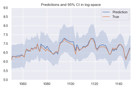
Not too bad, the mean squared error is 0.19 and the loss is -0.74 (remember we are subtracting the log of the variance, so the loss can be negative now). Applying the three steps outlined above gives:

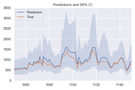
Notice how larger values are more stretched: this results in larger confidence intervals for predictions of larger magnitude, and equal error in log space become different after the exponential transformation. This is a direct consequence of this training procedure: the model is completely unaware of how large certain errors actually are, as the only thing it sees is the log space shown in the first graph. Hopefully it is clear by now: in log space, the errors are equal, but after exponentiation they can be very different.

Finally, this plot compares confidence intervals computed with the right and wrong methods:

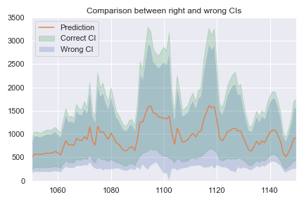
Notice how the confidence intervals have similar width: the correct confidence interval is a bit tighter, but the gap is only of a few percents when compared to the actual predictions. The big difference between the two methods is that the wrong confidence intervals are shifted down. In particular, they can contain negative values, which is very wrong.

References

1. Nix, D.A., and A.S. Weigend. Estimating the Mean and Variance of the Target Probability Distribution. In Proceedings of 1994 IEEE International Conference on Neural Networks (ICNN’94), 55–60 vol.1. Orlando, FL, USA: IEEE, 1994. ↩

2. Kendall, Alex, and Yarin Gal. What Uncertainties Do We Need in Bayesian Deep Learning for Computer Vision?, 5574–84, 2017. ↩ ↩²

3. De Vito, S., E. Massera, M. Piga, L. Martinotto, and G. Di Francia. On Field Calibration of an Electronic Nose for Benzene Estimation in an Urban Pollution Monitoring Scenario. Sensors and Actuators B: Chemical 129, no. 2 (February 2008): 750–57. ↩