The 37% rule
Suppose you want to pick the best item out of a collection, but you must decide after seeing each item whether to keep it and walk away or discard it and keep looking, loosing this item forever. An apartment search in competitive cities is an example of this kind of decision process. The optimal stopping rule is to examine the first 37% items without committing, then choose the item that is the best among the ones seen so far; incredibly, following this strategy one selects the absolute best item in 37% of the cases. But what happens when the best item is not selected?
This problem is also known as the secretary problem (where a boss has to pick the best candidate interviewing for a secretary position), and it is not hard to show that the optimal cutoff is $n/e\approx 0.3678\cdot n$ and the probability of selecting the best is also $1/e$. What is amazing is that this probability does not decrease with the number of items to choose from, so even if one could, for example, date the entire world population, they would end up choosing the best partner with a probability of 37%. Conveniently, when one does not have too many items to choose from, the probability of picking the best is even a bit higher, for example it is about 41% with ten items.
As I tend to be rather risk-averse, I could not help but wonder what happens when the best is not selected? In other words, what does an “average” choice looks like? Fortunately, this decision process is quite easy to simulate, for example in R:
choose37 <- function(ranks) {
  m <- as.integer(length(ranks) * exp(-1))
  best_of_m <- length(ranks)
  for(i in 1:length(ranks)) {
    r <- ranks[i]
    if(r < best_of_m) {
      if(i <= m) {
        best_of_m <- r
      }
      else {
        break
      }
    }
  }
  c(i, r)
}
This function takes as input the ranks of the items so that the best has rank
one. We can now simulate random set of items and choose according to this rule
simply via choose37(sample(n)). I then simulated 100,000 draws from 1,000
objects and computed statistics on the chosen rank.
These are the probabilities for the first ten ranks:
| Rank | Prob. |
|---|---|
| 1 | 0,368 |
| 2 | 0,137 |
| 3 | 0,0634 |
| 4 | 0,0311 |
| 5 | 0,0167 |
| 6 | 0,00832 |
| 7 | 0,0054 |
| 8 | 0,00324 |
| 9 | 0,00185 |
| Cum. | 0,63501 |
Therefore, the 37% rule will pick an item ranked in the top 1% with 63.5% probability. The distribution of ranks looks like this:
| Min. | 1st Qu. | Median | Mean | 3rd Qu. | Max. |
|---|---|---|---|---|---|
| 1 | 1 | 2 | 184.5 | 316 | 1,000 |
Even though in some cases we end up with the absolute worst item, on average we picked the top 18% and with 75% probability within the top 31.6%. That is not bad at all!
For a comprehensive picture, the (empirical) probability distribution looks like this:
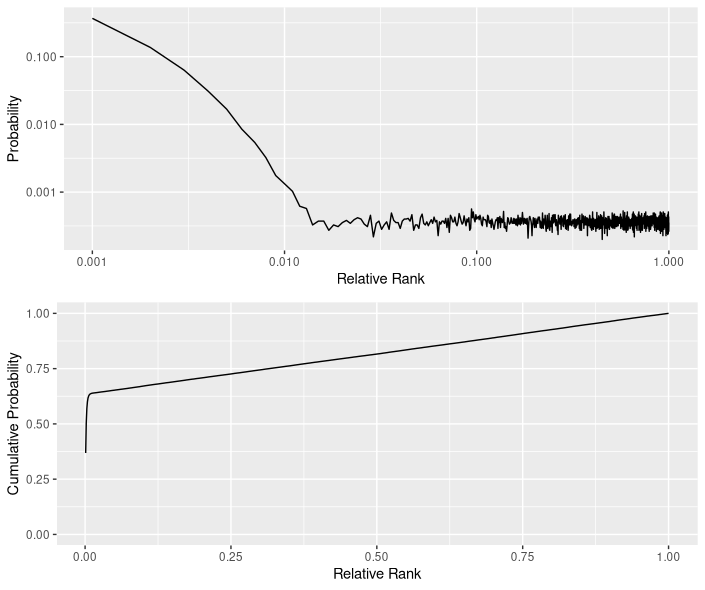
Quite interestingly, the distribution after rank 1.5% seems to be rather uniform, with a density that likely depends on the number of items.
In conclusion, the 37% rule works extremely well compared to its simplicity!