What is the average length of a queue of cars?

Some time ago I was driving on a twisty mountain road, stuck in a slow-moving queue of cars as it was impossible to overtake safely. Out of boredom, I was wondering how many cars were in the queue, and, more generally, what would be the average length of queues in this road. Let’s find out!

First, let’s formalize the problem. Assume that the road has a single entry, no exits, and is infinitely long (poor drivers!). Furthermore, upon entering the road each vehicle moves forward at a given average speed. In this scenario, faster vehicles will eventually catch up with the slower ones in front of them, and, since overtakes are not possible, will slow down and queue behind them. After some time, a “steady state” is reached where several groups of vehicles form, each moving forward at the speed of the slowest vehicle in front of the queue. The question we want to answer is, therefore: what is the average length of these groups?

The intuitive (but wrong) approach

The first idea I had was rather intuitive, but as it turns out, wrong. Let the average speeds of the $i$-th vehicle entering the road be $X_i$, and assume that all $X_1\ldots,X_\infty$ are independent and identically distributed (i.i.d.). Following our assumptions above, a queue of $n$ vehicles will form if $X_1\leq X_2$, and $X_1 \leq X_3$, and $\ldots$, and $X_1\leq X_n$, and $X_1>X_{n+1}$. Since all variables are i.i.d., we can find the probability of all of these events to be true as the product of the individual probabilities:

\[p(N=n)=\begin{cases} 1 & n \leq 1 \\ \left[\prod_{i=2}^n p(X_i\geq X_1)\right] p(X_{n+1}<X_1) & n \geq 2 \end{cases}\]

Some thought before going on with the math should convince you that the final result does not depend on the distributions of the velocities. Different distributions would affect how quickly queues form, but not their length after an infinite amount of time. Indeed, since $X_1$ and $X_i$ are i.i.d., the probability that $X_1\leq X_i$ must be $1/2$. Actually, for this we do not even need independence, but only exchangeability (which is implied by independence, and therefore holds in our case). In our case, exchangeable random variables have the property that $p(X_1=x,X_i=x’)=p(X_1=x’,X_i=x)$. This kind of symmetry means that there is no “preferred” ordering of the two velocities, and therefore the probability that one is larger than the other can only be $1/2$ (you can verify this formally by explicitly writing down and solving an integral for that probability).

Since $p(X_1\leq X_i)=1/2$, expanding the equation above gives:

\[p(N=n)= p(X_{n+1}<X_1)\prod_{i=2}^n p(X_i\geq X_1) = \frac{1}{2} \prod_{i=2}^n \frac{1}{2}=\frac{1}{2^{n-1}}\]

Which holds again for $n>1$; For example, there is a probability of $1/2$ that there are at least two cars. Finally, the expected value of $N$ is computed as

\[\mathbb{E}[N]=\sum_{n=1}^N n\cdot p(N=n)=\sum_{n=1}^N \frac{n}{2^n}=2\]

Therefore, the average number of cars in a queue is 2! Which definitely does not match my experience ;)

To conclude this (wrong, as we are going to see in a minute) solution, note that the derivation above was somewhat pedantic and brute-forced. With a little bit more insight, one could realize that, assuming the velocities to be i.i.d., the number of vehicles in a queue is a random variable with Geometric distribution. Each Bernoulli trial corresponds to a new vehicle entering the road and checking whether it is not faster than the queue of cars in front of it. A Geometric random variable with parameter $p=1/2$ has the same distribution and expectation that we derived above.

Simulation

As I hinted at the beginning, the reasoning above is actually wrong, and I only realized that because I implemented a simulation and found completely different results. Let’s dive in!

import seaborn as sns
from tqdm import trange
import matplotlib.pyplot as plt
import pandas as pd
import numpy as np

rnd = np.random.default_rng(2315)

First, we define a function to sample a random velocity $X_i$. For simplicity we sample from an uniform distribution, but you can easily change this one to verify that the average queue length does not depend on the distribution of the velocities.

def getv():
    ''' Returns the velocity of a random vehicle '''
    return rnd.uniform()

Next, we perform 100,000 simulations where we grow a queue as long as new cars are faster than the car in front:

sim_count = 100_000

queue_lengths = []
for _ in trange(sim_count):
    i, v0 = 1, getv()

    vi = getv()
    while vi >= v0:
        i += 1
        vi = getv()

    queue_lengths.append(i)

queue_lengths = np.array(queue_lengths)

100%|██████████| 100000/100000 [00:02<00:00, 33857.86it/s]

Let’s check some descriptive statistics of the queue lengths:

pd.Series(queue_lengths).describe()

count    100000.000000
mean         10.689810
std         200.154592
min           1.000000
25%           1.000000
50%           2.000000
75%           4.000000
max       22849.000000
dtype: float64

Half of the queues only contain two cars, as we also found above, however the average length of 11 cars is way off. Moreover, if the reasoning above was correct, observing a queue of 22,849 cars would be essentially impossible! Something is definitely wrong.

To confirm, let’s compare the empirical distribution of the queue lengths with our predictions:

plt.plot(
    sorted(queue_lengths),
    np.linspace(0, 1, len(queue_lengths)),
    label='Observed',
)

plt.step(
    np.arange(1, len(queue_lengths)),
    np.cumsum(0.5**np.arange(1, len(queue_lengths))),
    where='post',
    label='Computed',
)

plt.xscale('log')
plt.xlabel('Length')
plt.ylabel('CDF')
plt.legend()
plt.show()

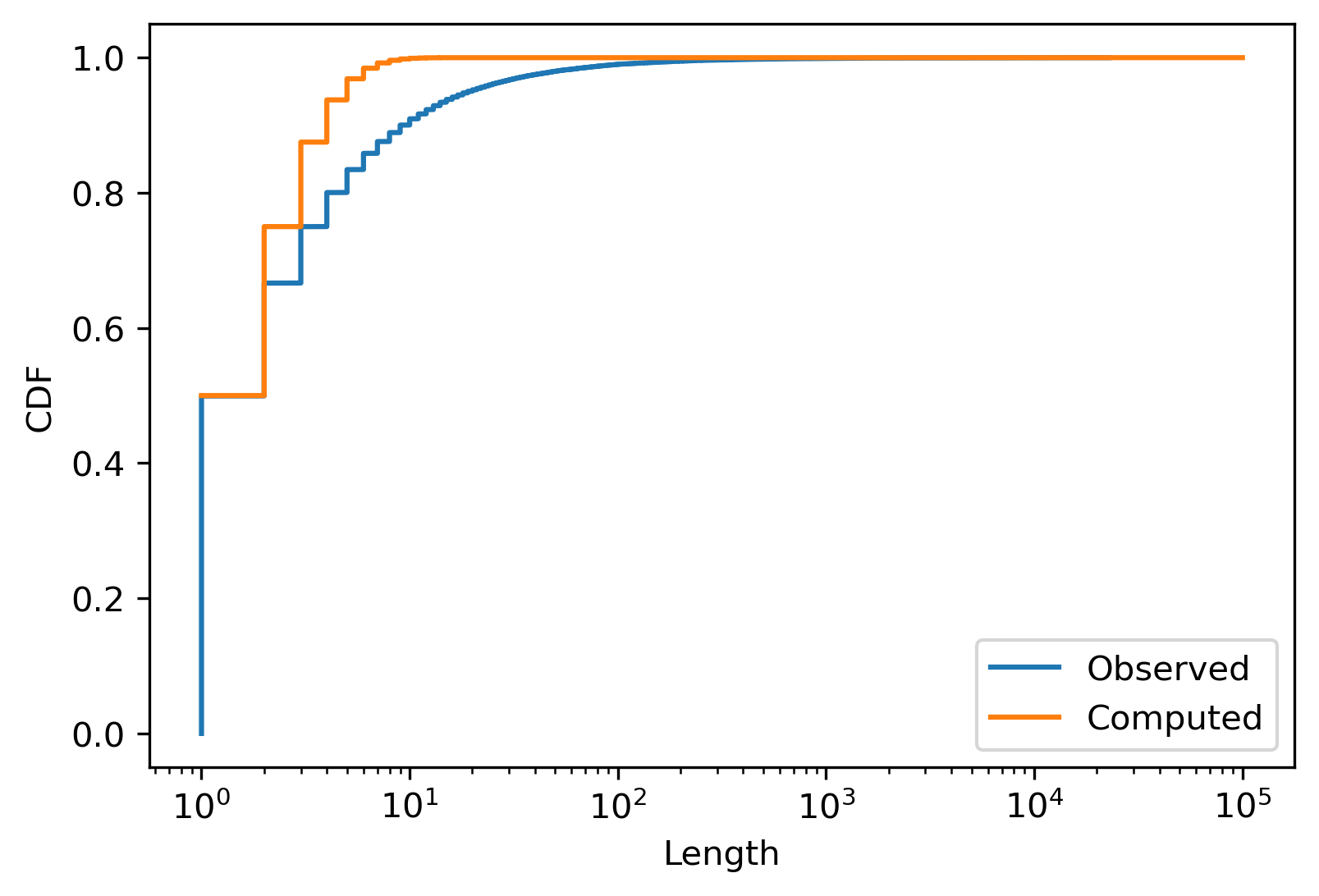
Except for the case of $n\leq 2$, we are way off, and the predicted probability of longer queues decays way too fast.

The Correct Solution

Finding the right solution took me a while. To be honest, even in this moment I am not really sure whether I understand why the reasoning above is wrong.

Consider this: if you see a queue of twenty cars, what can you infer about the car in front? It must be pretty slow compared to the average, right? But if the queue only has two cars, the one in front cannot be that slow, as compared to everybody else. In fact, suppose that the car in front is slower than 80% of all drivers. Then, each new driver entering the road has a probability of 80% to be faster than the car in front. Therefore, in that case, the probability that there are $n$ cars in a queue equals $0.8^{(n-1)}\cdot 0.2$, where the last term accounts for the fact that the last car entering the road is even slower than the first one. In formal terms, for $n>1$:

\[p(N=n\vert X_1=x)= \left[\prod_{i=2}^n p(X_i\geq x)\right] p(X_{n+1}<x)\]

Which should look familiar! It is indeed what we found above, except that now we are conditioning on the value of $X_1$. The reasoning based on exchangeability, while formally correct, does not apply to this problem because the first car of the queue is fixed.

We can remove the dependence on $x$ by integrating it away:

\[p(N=n)=\int_{-\infty}^{\infty} p(N=n|X_1=x)p(X_1=x)\text{d}x\]

At first sight, this mighty integral does not seem approachable due to the large product it contains. However, remember that all $X_i$’s are i.i.d., therefore we can simplify this expression as follows:

\[p(N=n\vert X=x)= \left[\prod_{i=2}^n p(X\geq x)\right]p(X<x) =p(X\geq x)^{n-1} p(X<x)\]

Since this only depends on the CDF of $X$, we can use the change of variable formula to get rid of the density of $X_1$, i.e., the term $p(X_1=x)$ in the integral above.

In general terms, the change of variable formula, or integration by substitution method, states that:

\[\int_a^b f(g(x))g'(x)\text{d}x=\int_{g(a)}^{g(b)}f(u)\text{d}u\]

where $u=g(x)$.

Here, we are going to use $u=g(x)=p(X\leq x)$, which means that $g’(x)=p(X=x)$, and obviously $f(g(x))=p(N=n|X=x)$. This makes $u$ an uniform random variable distributed between 0 and 1, and is known in statistics as the probability integral transform. With this substitution we obtain:

\[p(N=n)=\int_0^1 u (1-u)^{n-1} \text{d}u\]

If this transformation looks rather obscure to you, rest assured it is to me, too. But it is easy to justify it intuitively via the reasoning we did above: if the first car is in the slowest $u\%$ of all cars, then the probability that each new car is faster than that is $(1-u)\%$, and the probability of having $n$ cars in a queue is $u(1-u)^{n-1}$ (always accounting for the very last car that is even slower than the first one). And since we do not know what $u$ is, we have to try all possible values. We use the transformation above to work with quantiles instead of the actual velocity of the cars. This has a beautiful consequence:

Our results hold no matter what is the distribution of car velocities. In other words, no amount of driving lessons or better roads can influence the length of queues (assuming that roads are long enough for queues to grow).

To solve this we perform another change of variable with $v=1-u$ and $\text{d}u=-\text{d}v$ to obtain:

\[p(N=n)=\int_1^0 -(1-v) v^{n-1} \text{d}v=\int_1^0\left(v^n-v^{n-1}\right)\text{d}v\]

Now, the two pieces can be approached independently: given that the indefinite integral of $v^n$ is $v^{n+1}/(n+1)$, the solution is

\[p(N=n)= \frac{v^{n+1}}{n+1}\bigg\vert_1^0 -\frac{v^{n}}{n}\bigg\vert_1^0 =-\frac{1}{n+1}+\frac{1}{n} =\frac{1}{n(n+1)}\]

Before doing anything else, let’s compare this result with our earlier simulation:

plt.plot(
    sorted(queue_lengths),
    np.linspace(0, 1, len(queue_lengths)),
    label='Observed',
)

plt.step(
    np.arange(1, len(queue_lengths)),
    np.cumsum([1/(n*(n+1)) for n in range(1,len(queue_lengths))]),
    where='post',
    label='Computed',
)

plt.xscale('log')
plt.xlabel('Length')
plt.ylabel('CDF')
plt.legend()
plt.show()

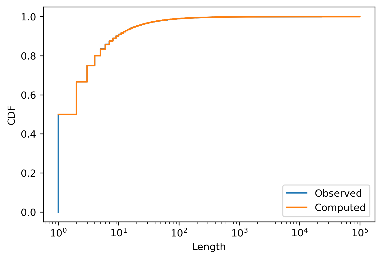
They match beautifully! Here is another way of comparing the two distributions:

n = 50
plt.plot(
    1-np.cumsum([1/(n*(n+1)) for n in range(1,n)]),
    [1-np.mean(np.array(queue_lengths) <= i) for i in range(1,n)],
    'o'
)
plt.plot([0., .5], [0, .5], '--', label='y=x')
plt.xscale('log')
plt.yscale('log')
plt.xlabel('Observed probability')
plt.ylabel('Computed probability')
plt.legend()
plt.show()

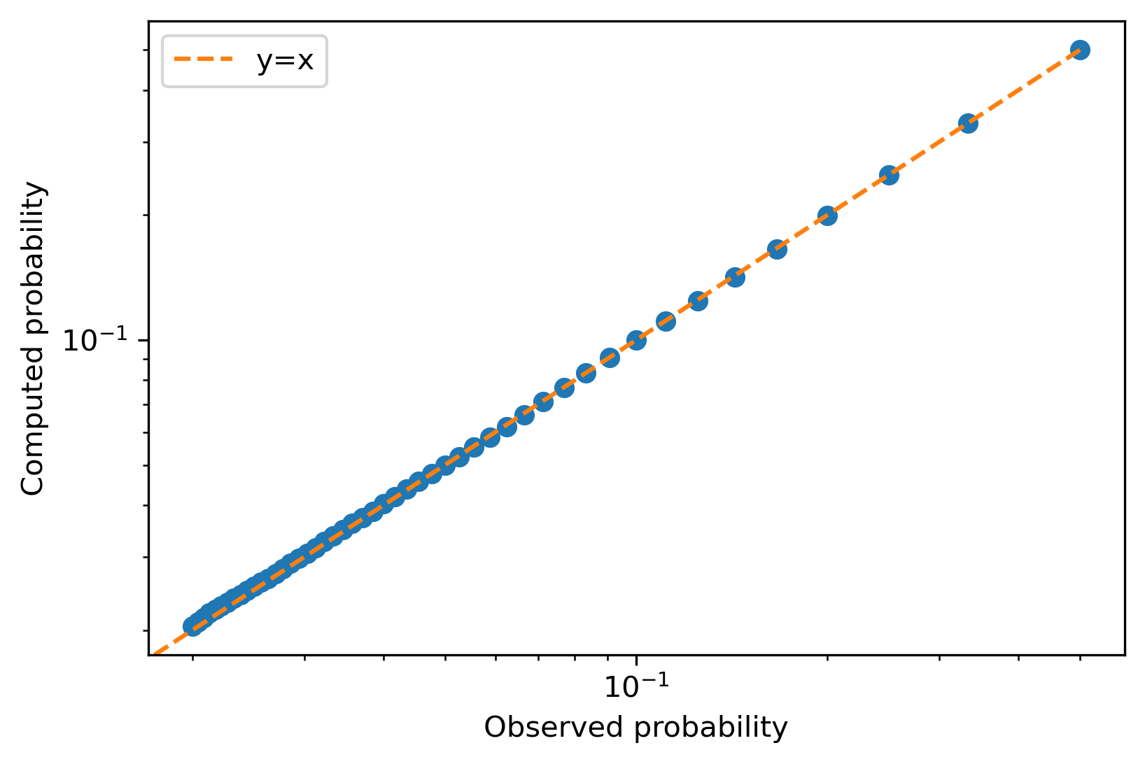
In this chart, each dot is a specific queue length, and the $x$ and $y$ values are the observed and computed probabilities of a queue having that length. Again, we see great agreement.

Now that we are confident that we have a formula for distribution of the queue length, let’s compute its expected value:

\[\mathbb{E}[N]=\sum_{n=1}^\infty n\cdot p(N=n)=\sum_{n=1}^\infty \frac{n}{n(n+1)} =\sum_{n=1}^\infty \frac{1}{n+1}\]

Uh oh. This series diverges to infinity.

I am afraid that long queues will exist even in the most advanced alien society (as long as they are based on roads).