Limits of single-hidden-layer neural networks
A few decades ago, researchers were trying to understand which kind of shapes can be modeled by neural networks. Even after the universal approximation theorem was proven, they still wanted to know which kind of decision regions (i.e. regions in the input space classified as positive) can be exactly reproduced, and which ones can only be approximated, with a neural network with a single hidden layer.
Before the activation, a neuron defines a hyper-plane in its input space, and assigns positive value to points on one side and negative value to points on the other side. The exact value depends on the distance of the point from this hyper-plane, as well as the magnitude of the weights of the neuron. Then, the activation function simply scales this value; in this discussion we will always use the threshold activation, i.e. one if positive and zero if negative.
If every neuron defines a hyper-plane, several neurons will partition the input space into a number of polyhedral sets, and every input point inside one of these sets would generate the same activations in the hidden neurons. This must be so, because they are all on the same side of every hyper-plane, and the network would only be able to differentiate points belonging to different regions. In other words, there can only be one label per region.
For every input point, the hidden layer would output a binary vector identifying which region the point is in. This binary vector would be one of the vertices of a $d$-dimensional hyper-cube, where $d$ is the size of the hidden layer. Just like the neurons in the hidden layer, the single output neuron would define another hyper-plane in this $d$-dimensional space, classifying the hidden activation patterns on one side as positive, and negative on the other side.
An example would definitely help:

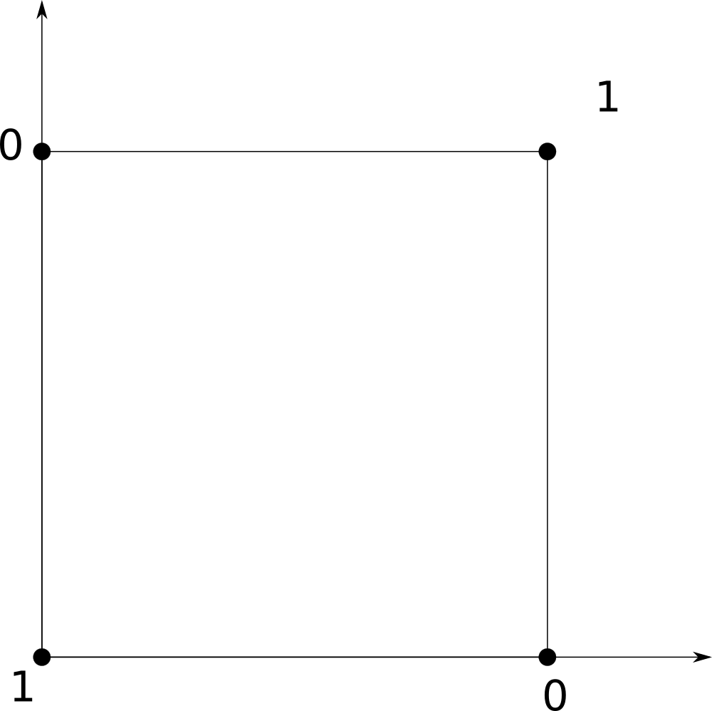
Here we have two neurons that define two lines, L1 and L2. The neuron corresponding to L1 predicts one for points “above” the line, while the other neuron predicts one for points to the right of L2. Together, these two lines split the input space into four regions, and each region causes a different activation pattern in the neurons (represented by the two numbers in parenthesis). You can imagine these four regions as the vertices of a square, as the activation patterns indicate one of these vertices. Then, we can carry over the labels from the input space to this new space of the hidden neurons, and the process repeats all over again with the neurons in the next layer. Now, the same reasoning applies to an arbitrary number of input and hidden neurons, it just becomes harder to visualize.
Towards the end 1990, a paper1 came up with one examples of decision regions that could not be reproduced with a single hidden layer. The proof was based on the concepts I explained above: they found a specific arrangement of lines that would result in a certain labeling in the input space that could not be linearly separated by the output neuron. This example is actually very simple, it is the picture above! Imagine that you want to label all the points in the (0,0) and (1,1) regions as 1, and the points in (0,1) and (1,0) as 0. The hidden space would be:
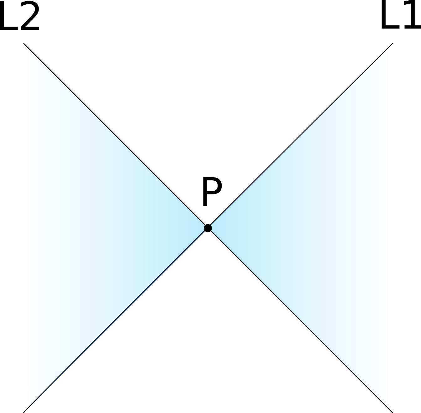
This is exactly the XOR problem! And we know that a perceptron (i.e., our output neuron) cannot solve this. Now, the proof is obviously a bit more technical, but this is the idea. Hence, any decision region that looks like the image below, where we predict one for the blue regions and zero for the other, cannot be modeled exactly.
A few months later, another paper2 proposed a different proof of this fact, which I find much more intuitive even though it uses some (trivial) math. Consider four points in the four regions of the image above:
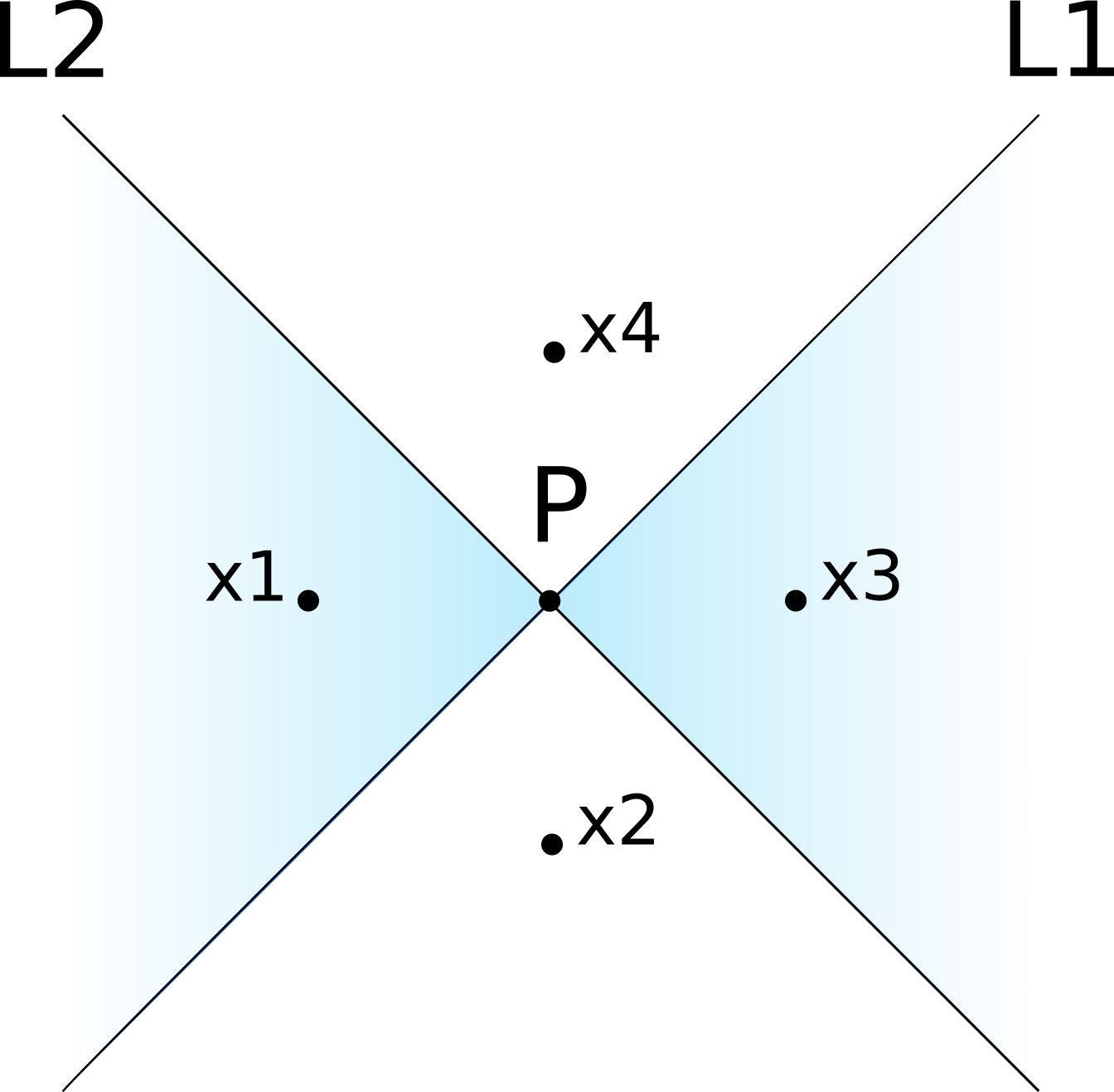
And assume that there actually is a one-hidden-layer neural network $g$ that can perfectly reproduce that decision region, so that $g(\textbf{x}_1)=g(\textbf{x}_3)=1$ and $g(\textbf{x}_2)=g(\textbf{x}_4)=0$. Now consider the difference between the predictions for $x_1$ and $x_2$:
\[\begin{align*} g(\textbf{x}_1)-g(\textbf{x}_2) &= \sum_{i=1}^m w_i\cdot \sigma(\textbf{x}_1^T\textbf{v}_i+c_i)+b -\sum_{i=1}^m w_i\cdot \sigma(\textbf{x}_2^T\textbf{v}_i+c_i)-b \\ &= w_1\cdot \sigma(\textbf{x}_1^T\textbf{v}_1+c_1)-w_1\cdot \sigma(\textbf{x}_2^T\textbf{v}_1+c_1) \\ & =w_1\cdot 0-w_1\cdot 1 \\ &= -w_1 \end{align*}\]This means that $w_1=-1$, because $g(\textbf{x}_1)-g(\textbf{x}_2)=1$ as we assumed above. You can do exactly the same reasoning for the other two points, and you would obtain the same result:
\[\begin{align*} g(\textbf{x}_4)-g(\textbf{x}_3) &=w_1\cdot \sigma(\textbf{x}_4^T\textbf{v}_1+c_1)-w_1\cdot \sigma(\textbf{x}_3^T\textbf{v}_1+c_1)) \\ &=-w_1 \end{align*}\]Except that $g(\textbf{x}_4)-g(\textbf{x}_3)=-1$, which implies that $w_1=1$! As we reached a contradiction, such a neural network does not exist.
This proof is, after all, equivalent to the previous one, but why do I find it more intuitive? Well, when you go from $\textbf{x}_1$ to $\textbf{x}_2$ you only cross L1, and you move from a region that has output zero to a region that has output one. When you go from $\textbf{x}_4$ to $\textbf{x}_3$ you move in the same direction and you also cross L1 only, except that now you go from a “zero” region to a “one” region. In both cases, you move from one side of L1 to the other, and nothing else changes, yet somehow the predictions are different, which is clearly impossible.
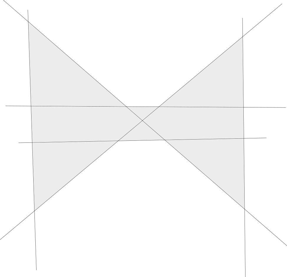
But the universal approximation theorem assures us that no matter the decision region, you can get as close as you want. So how can you approximate the bow tie? Here is how:
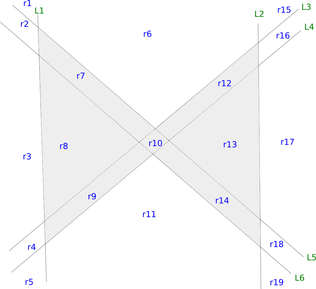
As L3 gets closer to L4, and L5 to L6, you will recover the bow tie figure. These six lines define a total of 19 regions, of which the gray ones should be classified positive and the remaining negative. The quickest way to prove this is possible is to fit a logistic regression model! The dataset would be the following:
| r | L1 | L2 | L3 | L4 | L5 | L6 | y |
|---|---|---|---|---|---|---|---|
| r1 | 0 | 0 | 1 | 1 | 1 | 1 | 0 |
| r2 | 0 | 0 | 1 | 1 | 0 | 1 | 0 |
| r3 | 0 | 0 | 1 | 1 | 0 | 0 | 0 |
| r4 | 0 | 0 | 0 | 1 | 0 | 0 | 0 |
| r5 | 0 | 0 | 0 | 0 | 0 | 0 | 0 |
| r6 | 1 | 0 | 1 | 1 | 1 | 1 | 0 |
| r7 | 1 | 0 | 1 | 1 | 0 | 1 | 1 |
| r8 | 1 | 0 | 1 | 1 | 0 | 0 | 1 |
| r9 | 1 | 0 | 0 | 1 | 0 | 0 | 1 |
| r10 | 1 | 0 | 0 | 1 | 0 | 1 | 1 |
| r11 | 1 | 0 | 0 | 0 | 0 | 0 | 0 |
| r12 | 1 | 0 | 0 | 1 | 0 | 1 | 1 |
| r13 | 1 | 0 | 0 | 0 | 0 | 1 | 1 |
| r14 | 1 | 0 | 0 | 0 | 0 | 1 | 1 |
| r15 | 1 | 1 | 1 | 1 | 1 | 1 | 0 |
| r16 | 1 | 1 | 0 | 1 | 1 | 1 | 0 |
| r17 | 1 | 1 | 0 | 0 | 1 | 1 | 0 |
| r18 | 1 | 1 | 0 | 0 | 0 | 1 | 0 |
| r19 | 1 | 1 | 0 | 0 | 0 | 0 | 0 |
Where there is a sample for every region and a feature for every line; one means “above” and/or “right” of that line. The weights associated to the regions one through six are 1.75, -1.5, -0.25, 0.5, -1.5 and 0.5, with bias of -2. As these regions are linearly separable, a neural network with one hidden layer is able to learn to separate gray from white regions in the image above.
The image below shows a way to approximate the bow tie that cannot be learned:
Where the idea is that the bow tie can be approximated arbitrarily well by moving the two horizontal lines closer to the center. Unfortunately, these eight regions cannot be separated linearly.