Automatic differentiation from scratch
Automatic differentiation (AD) is one of the most important features present in modern frameworks such as Tensorflow, Pytorch, Theano, etc. AD has made paramter optimization through gradient descent an order of magnitude faster and easier, and drastically lowered the barrier of entry for people without a solid mathematical background. In spite of its utility, AD is surprisingly simple to implement, which is what we are going to do here.
AD is based on a computational graph. This is a directed acyclic graph whose nodes are variables and operations on these variables, and whose edges connect an operation to its operands. Consider the very simple expression:
\[z=x^2+3xy + 1\]This can be associated to the following graph:
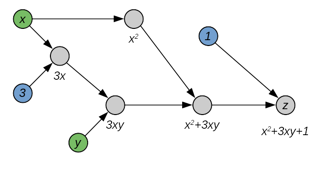
In this graph, we can distinguish three types of nodes: blue nodes are constants, green nodes are variables, and gray nodes are operation nodes. Every operation node, as the name says, performs a specific operation on the incoming nodes. Some nodes can be named explicitly by being associated to a variable.
Once we have such a graph, computing derivatives can be done recursively via the chain rule:
\[\frac{\text{d}}{\text{d}x}f(g(x))=\frac{\text{d}}{\text{d}g}f(g(x))\cdot \frac{\text{d}}{\text{d}x}g(x)\]Where $f$ and $g$ are two nodes in the computational graph, and $g$ is connected to $f$. The formula simply says that to differentiate $f$ with respect to $x$, we must recursively apply the same formula to $g$, then multiply the result with the derivative of $f$ with respect to its argument.
An example will make it clear: suppose that $g(x)=3x$ and $f(x)=x^2$, then:
\[\frac{\text{d}}{\text{d}x}g(x)=3\] \[\frac{\text{d}}{\text{d}x}f(x)=2x\]Therefore:
\[\frac{\text{d}}{\text{d}g}f(g(x))=3\cdot2x\]and:
\[\frac{\text{d}}{\text{d}x}f(g(x))=\frac{\text{d}}{\text{d}g}f(g(x))\cdot \frac{\text{d}}{\text{d}x}g(x)=3\cdot(2x)\cdot 3=18x\]For generic function of several parameters, we have to implement the total derivative, which, stated simply, is:
\[\frac{\text{d}}{\text{d}x} f(g(x), h(x))= \frac{\text{d}}{\text{d}g}f(g(x),h(x))\cdot\frac{\text{d}}{\text{d}x}g(x) +\frac{\text{d}}{\text{d}h}f(g(x),h(x))\cdot\frac{\text{d}}{\text{d}x}h(x)\]Or, less explicit but easier to read:
\[\frac{\text{d}f}{\text{d}x}=\frac{\text{d}f}{\text{d}g}\frac{\text{d}g}{\text{d}x}+\frac{\text{d}f}{\text{d}h}\frac{\text{d}h}{\text{d}x}\]In other words, we simply sum the derivatives of the arguments with respect to $x$.
Again, an example will clear this up. Suppose that $g(x)=3x$, $h(x)=x^2$ and $f(x,y)=xy$, so that $f(g(x),h(x))=(3x)(x^2)=3x^3$. The individual derivatives are:
\[\frac{\text{d}g}{\text{d}x}=3\] \[\frac{\text{d}h}{\text{d}x}=2x\] \[\frac{\text{d}f}{\text{d}g}=h\] \[\frac{\text{d}f}{\text{d}h}=g\]Putting these together, we get:
\[\frac{\text{d}f}{\text{d}x}=\frac{\text{d}f}{\text{d}g}\frac{\text{d}g}{\text{d}x}+\frac{\text{d}f}{\text{d}h}\frac{\text{d}h}{\text{d}x}=(x^2)3+(3x)(2x)=3x^2+6x^2=9x^2\]which is what we expected.
Implementation
Let us now implement this mechanism, I promise it is easier than it looks like. We first create an abstract class for nodes:
from abc import ABC, abstractmethod
class DifferentiableSymbolicOperation(ABC):
    @abstractmethod
    def backward(self, var):
        pass

    @abstractmethod
    def compute(self):
        pass
Where the first method, backward, will return a new DifferentiableSymbolicOperation. This will make it easy to compute second derivatives, third derivatives, and so on. The second method, compute, will perform the actual computations and return a numerical result.
Next, we implement a node for constants:
class Const(DifferentiableSymbolicOperation):
    def __init__(self, value):
        self.value = value

    def backward(self, var):
        return Const(0)

    def compute(self):
        return self.value

    def __repr__(self):
        return str(self.value)
The value of a constant is simply the value we decided, and its derivative with respect to any variable is zero:
\[\frac{\text{d}}{\text{d}x} k=0\]Notice that backward constructs new nodes, it does not perform the actual operations. In this way, we will have a new computational graph representing the derivative with respect to the variable. Finally, we use __repr__ to construct a string representation of the expression, so that we can easily inspect the graph.
Variable nodes are also simple:
class Var(DifferentiableSymbolicOperation):
    def __init__(self, name, value=None):
        self.name, self.value = name, value

    def backward(self, var):
        return Const(1) if self == var else Const(0)

    def compute(self):
        if self.value is None:
            raise ValueError('unassigned variable')
        return self.value

    def __repr__(self):
        return f'{self.name}'
Where the derivative is one if this is the variable we are differentiating on, otherwise zero, as it can be regarded as a constant. In mathematical notation:
\[\frac{\text{d}}{\text{d}x}x=1\] \[\frac{\text{d}}{\text{d}x}y=0\]We can now implement a node for addition:
class Sum(DifferentiableSymbolicOperation):
    def __init__(self, x, y):
        self.x, self.y = x, y

    def backward(self, var):
        return Sum(self.x.backward(var), self.y.backward(var))

    def compute(self):
        return self.x.compute() + self.y.compute()

    def __repr__(self):
        return f'({self.x} + {self.y})'
This is where things start to become interesting: to take the derivative of $f(x)+g(x)$ we simply sum the two individual derivatives. In case $x$ does not appear in $f$ or $g$, we will get zero, as expected. We do not need to multiply by $\text{d}f/\text{d}x$ here, because this is already done in self.x.backward(). To compute the sum, we recursively compute the values of the incoming nodes, and add them together.
The product node is implemented as follows:
class Mul(DifferentiableSymbolicOperation):
    def __init__(self, x, y):
        self.x, self.y = x, y

    def backward(self, var):
        return Sum(
            Mul(self.x.backward(var), self.y),
            Mul(self.x, self.y.backward(var))
        )

    def compute(self):
        return self.x.compute() * self.y.compute()

    def __repr__(self):
        return f'({self.x} * {self.y})'
As you can see, this translates exactly to the rule for derivating products you learned in high school. With these simple ingredients, we can already model the expression we had above:
\[z=x^2+3xy + 1\]x = Var('x', 3)
y = Var('y', 2)
z = Sum(
Sum(
Mul(x, x),
Mul(Const(3), Mul(x, y))
),
Const(1)
)
z
(((x * x) + (3 * (x * y))) + 1)
It is a bit cumbersome, but it seems to work. Let us try to compute the value of $z$ when $x=3$ and $y=2$:
z.compute(), 3**2 + 3*3*2 + 1
(28, 28)
The results match. Now let us differentiate with respect to $x$:
z.backward(x)
((((1 * x) + (x * 1)) + ((0 * (x * y)) + (3 * ((1 * y) + (x * 0))))) + 0)
We can simplify this expression to get the result we expected:
\[\frac{\text{d}z}{\text{d}x}=1\cdot x + x\cdot 1 + 0\cdot xy + 3\cdot(1\cdot y+x\cdot 0)+0=x+x+3y=2x+3y\]And, obviously, we can compute the value of this derivative with the actual values of $x$ and $y$:
z.backward(x).compute()
12
Which certainly equals $2\cdot 3+3\cdot 2$. And, to show-off, here’s a mixed partial derivative:
z.backward(x).backward(y)
(((((0 * x) + (1 * 0)) + ((0 * 1) + (x * 0))) + (((0 * (x * y)) + (0 * ((0 * y) + (x * 1)))) + ((0 * ((1 * y) + (x * 0))) + (3 * (((0 * y) + (1 * 1)) + ((0 * 0) + (x * 0))))))) + 0)
This is a bit harder to read, and certainly not very efficient to compute since we have so many zeros.
Graph optimization
Luckily, it is easy to write a recursive function that simplifies expressions, and we can go a long way with simple rules.
def simplify(node):
    if isinstance(node, Sum):
        return simplify_sum(node)
    elif isinstance(node, Mul):
        return simplify_mul(node)
    else:
        return node
We can now write these functions and apply the relevant simplifications, such as $x+0=x$. A second simplification is when both operands are constants, we can perform the summ immediately.
def simplify_sum(node):
    # first, recursively simplify the children
    x = simplify(node.x)
    y = simplify(node.y)

    x_const = isinstance(x, Const)
    y_const = isinstance(y, Const)

    if x_const and y_const:
        # propagate constants
        return Const(x.value + y.value)
    elif x_const and x.value == 0:
        # 0 + y = y
        return y
    elif y_const and y.value == 0:
        # x + 0 = x
        return x
    else:
        # return a new node with the simplified operands
        return Sum(x, y)
A quick test:
(
    simplify_sum(Sum(x, Const(0))),
    simplify_sum(Sum(Const(2), Const(3)))
)
(x, 5)
Products can be simplified similarly:
def simplify_mul(node):
    # first, recursively simplify the children
    x = simplify(node.x)
    y = simplify(node.y)

    x_const = isinstance(x, Const)
    y_const = isinstance(y, Const)

    if x_const and y_const:
        # propagate constants
        return Const(x.value * y.value)
    elif x_const and x.value == 0:
        # 0 * y = 0
        return Const(0)
    elif x_const and x.value == 1:
        # 1 * y = 1
        return y
    elif y_const and y.value == 0:
        # x * 0 = 0
        return Const(0)
    elif y_const and y.value == 1:
        # x * 1 = 1
        return x
    else:
        # return a new node with the simplified operands
        return Mul(x, y)
Let us test this simplification on the derivatives we computed earlier:
simplify(z.backward(x))
((x + x) + (3 * y))
Note that simplifying f(x)+f(x) into 2f(x) is not trivial in the general case, because we first need to establish that the two sides are mathematically equivalent. A bit more restrictively, we could check if the trees are identical, node-by-node.
Finally, the mixed derivative $\text{d}^2z/\text{d}x\text{d}y$ of our running example is:
simplify(z.backward(x).backward(y))
3
As expected. By the way, do not forget that this is a node:
type(simplify(z.backward(x).backward(y)))
__main__.Const
From a software engineering perspective, a better approach to implement this would be to add a new abstract method to DifferentiableSymbolicOperation, and let each class implement its own simplifications. For example, an Exp class could implement the rule Exp(Const(0))=1.
Improving the user experience
Currently, users would need to explicitly use Const, Sum and Mul for every operation. This gets tedious very quickly. We would like to imitate the big frameworks, and let users use the normal Python operators +, *, etc. This is also easy to achieve, by implementing specific methods in our node classes.
Since the implementation would be the same for every node type, we can reduce code duplication through a mixin:
class ErgonomicNodeMixin:
    @staticmethod
    def _to_symbolic(x):
        '''
        makes sure that x is a tree node by converting it
        into a constant node if necessary
        '''
        if not isinstance(x, DifferentiableSymbolicOperation):
            return Const(x)
        else:
            return x

    def __add__(self, other):
        return ErgonomicSum(self, self._to_symbolic(other))

    def __mul__(self, other):
        return ErgonomicMul(self, self._to_symbolic(other))

    def __neg__(self):
        return ErgonomicMul(Const(-1), self)
We can now create the actual “ergonomic” classes:
class ErgonomicVar(Var, ErgonomicNodeMixin):
    pass

class ErgonomicSum(Sum, ErgonomicNodeMixin):
    pass

class ErgonomicMul(Mul, ErgonomicNodeMixin):
    pass
Our running example is now much easier to express:
x = ErgonomicVar('x', 3)
y = ErgonomicVar('y', 3)

z = x * x + x * y * 3 + 1

z.backward(x)
((((1 * x) + (x * 1)) + ((((1 * y) + (x * 0)) * 3) + ((x * y) * 0))) + 0)
Had we inserted the simplify method in each class, we would also be able to simplify this with no additional changes.
Logistic regression, from scratch and without gradients
It is now time to put our auto differentiation library to the test! I collected everything into a module, and implemented subtraction, division, natural exponentiation and logarithm with the relative optimizations and user experience improvements.
# our own automatic differentiation library!
# download from https://e-dorigatti.github.io/attachments/autodiff.py
import autodiff as ad
from sklearn import datasets
from sklearn.linear_model import LogisticRegression
from sklearn.metrics import confusion_matrix
import matplotlib.pyplot as plt
import math, random
import numpy as np

random.seed(12345)
We will use the iris dataset from scikit-learn. Here we normalize the inputs and encode the outputs as one-hot vectors. Note that we are not using a separate validation set in this case because we are only interested in the optimization procedure. In other words, generalization is not our concern here.
iris = datasets.load_iris()
x_train = iris['data']
x_train = (x_train - x_train.mean(axis=0)) / x_train.std(axis=0)
y_train = np.zeros((x_train.shape[0], 3))
for i, y in enumerate(iris['target']):
    y_train[i][y] = 1.0
We now implement a softmax regression model:
\[z_i = b_i+\sum_j x_jw_{ij}\] \[\hat{y}_{i}=\frac{\exp(z_i)}{\sum_j \exp(z_j)}\]With the usual cross entropy loss:
\[\mathcal{L}(\textbf{y}, \hat{\textbf{y}})=\sum_i y_i\log\hat{y}_i\]Here we try to imitate scikit’s API, with the methods fit, predict and predict_proba:
class SoftmaxRegression:
    def __init__(self, input_shape, num_classes, l2, epochs, batch_size, base_lr):
        self._input_shape = input_shape
        self._num_classes = num_classes
        self._epochs = epochs
        self._batch_size = batch_size
        self._base_lr = base_lr

        # these variables are just placeholders for the input features
        # of an individial input sample
        self._inputs = [ad.Var(f'x_{i}') for i in range(input_shape)]

        # create the parameters and the pre-softmax outputs for each class
        self._params, self._biases, self._logits, self._labels = [], [], [], []
        for i in range(num_classes):
            # parameters needed to compute z_i
            b = ad.Var(f'b_{i}', value=0)
            ws = [
                ad.Var(f'w_{i}_{j}', value=random.gauss(0, 0.1))
                for j in range(input_shape)
            ]

            # output of the linear model
            z_i = b + sum(w * x for w, x in zip(ws, self._inputs))

            # placeholder for the true label to compute the loss
            y = ad.Var(f'y_{i}')

            self._params.extend(ws)
            self._params.append(b)
            self._logits.append(z_i)
            self._labels.append(y)

        # compute the softmax output
        softmax_norm = sum(ad.Exp(m) for m in self._logits)
        self._outputs = [ad.Exp(l) / softmax_norm for l in self._logits]

        # and the cross entropy loss
        self._loss = -sum(
            l * ad.Log(o + 1e-6) for l, o in zip(self._labels, self._outputs)
        ) + l2 * sum(w * w for w in self._params)

        # finally, compute the gradients for each parameter
        self._grads = [self._loss.backward(p).simplify() for p in self._params]

    def fit(self, X, y):
        ''' trains the model on the given data '''
        history = []
        batch_count = 0
        for epoch in range(self._epochs):
            idx = np.random.permutation(X.shape[0])
            for i in range(0, len(X), self._batch_size):
                batch_idx = idx[i:i+self._batch_size]
                loss = self._sgd_step(
                    X[batch_idx], y[batch_idx],
                    lr=self._base_lr / math.sqrt(1 + epoch)
                )
                history.append(loss)

            if epoch % 10 == 0:
                print(f'epoch: {epoch}\tloss: {loss:.3f}')

        return history

    def _sgd_step(self, batch_x, batch_y, lr):
        '''perform one step of stochastic gradient descent '''

        # here we accumulate gradients and loss
        grad_acc = [0.0] * len(self._grads)
        loss_acc = 0.0
        for x, y in zip(batch_x, batch_y):
            # set input and output placeholders to the values of this sample
            for input_, value in zip(self._inputs, x):
                input_.value = value
            for label_, value in zip(self._labels, y):
                label_.value = value

            # accumulate loss and gradients
            loss_acc += self._loss.compute()
            for i, g in enumerate(self._grads):
                grad_acc[i] += g.compute()

        # average the gradients and modify the parameters
        for p, g in zip(self._params, grad_acc):
            p.value = p.value - lr * g / len(batch_x)

        # return average loss for this minibatch
        return loss_acc / len(batch_x)

    def predict_proba(self, batch_x):
        ''' predict the class probabilities for each input sample in a batch '''
        preds = []
        for x in batch_x:
            # set input placeholders
            for input_, value in zip(self._inputs, x):
                input_.value = value

            # compute output probability for each class
            preds.append([o.compute() for o in self._outputs])

        return preds

    def predict(self, batch_x):
        ''' predict the class of each output sample '''
        probs = self.predict_proba(batch_x)
        return [
            max(enumerate(ps), key=lambda x: x[1])[0]
            for ps in probs
        ]
This is not too different from Tensorflow 1.x, where you first build the graph and all the operations needed, then use these operations during optimization. The biggest difference is that the optimizer in Tensorflow is also part of the graph, while in our implementation the gradients are accumulated outside of the graph, and the values of the weights overwritten with the new values. In practice, this would be quite expensive, for example when the variables are stored in the GPU memory, as we would be constantly moving a whole model’s worth of data in and out of the GPU several times for each batch. To amend this, we would need to implement an assignment operator directly in the graph.
It is time to fit and test our model:
model = SoftmaxRegression(
input_shape=len(x_train[0]), num_classes=len(y_train[0]),
l2=1e-6, epochs=100, batch_size=32, base_lr=5e-2
)
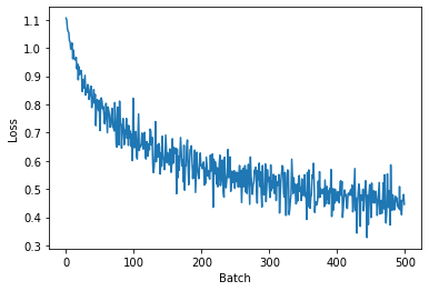
history = model.fit(x_train, y_train)
epoch: 0	loss: 1.055
epoch: 10	loss: 0.785
epoch: 20	loss: 0.619
epoch: 30	loss: 0.613
epoch: 40	loss: 0.514
epoch: 50	loss: 0.507
epoch: 60	loss: 0.528
epoch: 70	loss: 0.487
epoch: 80	loss: 0.504
epoch: 90	loss: 0.494
plt.plot(history)
plt.xlabel('Batch')
plt.ylabel('Loss')
plt.show()
Let’s see how good is our classifier on the training data:
preds = model.predict(x_train)
from sklearn.metrics import confusion_matrix
confusion_matrix(iris['target'], preds)
array([[50,  0,  0],
       [ 0, 31, 19],
       [ 0,  2, 48]])
(preds == iris['target']).mean()
0.86
Accuracy of 86% (on the training set), and perfect predictions for the first class, while the second class is frequently mistaken for the third. In terms of classification performance there is a lot of room for improvement, but we covered a lot of ground today already!
Summary
Automatic differentiation is extremely useful and one of the main reasons behind the recent boom in popularity of deep learning. In spite of its benefits, it is also very easy to implement, at least conceptually. Essentially, once one has a graph representing the desired computations, the derivatives can be computed recursively by using the chain rule. In this blog post, we implemented this from scratch and tested our implementation by creating and optimizing a softmax regression model on the iris dataset.