Simplest Implementation of Diffusion Models
This tutorial presents the simplest possible implementation of diffusion models in plain pytorch, following the exposition of Ho 2020, Denoising Diffusion Probabilistic Models.1
Generative models learn to generate new samples (e.g., images) starting from a latent variable following a tractable (i.e., simple) distribution. Diffusion models have recently emerged as a very powerful and capable type of generative models, underlying most of the latest astonishing examples of generative AI that have captured public imagination, such as Stable Diffusion,2 Midjourney,3 and DALL.E4. Diffusion models do this by first establishing a simple way to transform samples from the distribution of interest (the images) to a Gaussian distribution, then training a neural network to reverse this process. In this way, the network learns how to transform samples from the Gaussian into samples from the distribution of interest.
Diffusion refers to the gradual corruption of training examples by repeatedly adding a small amount of noise, mimicking the way heat diffuses through a material until it reaches an uniform temperature. After a few hundreds or thousands of noise diffusion steps, the information in the original sample is completely lost, such that the result is indistinguishable from the Gaussian that we will use as a starting point to generate new samples. Figure 2 from the paper (Ho, 2020) demonstrates this process graphically:
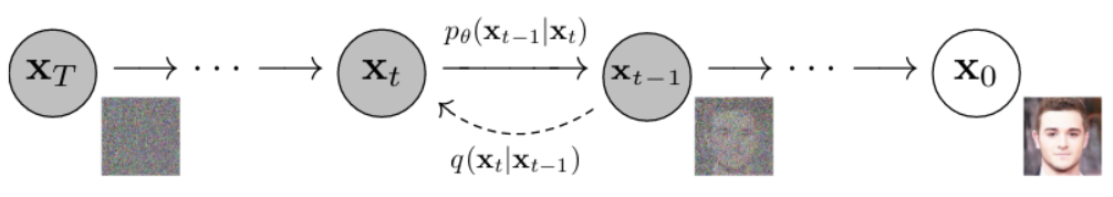
Here, $x_0$ is the original sample, the image of a guy, and the process of adding noise is represented by the dashed arrow going from right to left, so that, after $T$ steps, only noise remains in $x_T$. The generative process is represented by the arrows going from left to right, from $x_T$ to $x_0$, and the generative model is denoted by $p_\theta$, while the noise-adding process is $q$.
In this tutorial, we will learn to generate samples from a very simple unidimensional distribution, so that we can easily visualize the generative process. Let’s start by generating some data:
import matplotlib.pyplot as plt
import matplotlib as mpl
import pandas as pd
import numpy as np
import torch
import seaborn as sns
import itertools
from tqdm.auto import tqdm
data_distribution = torch.distributions.mixture_same_family.MixtureSameFamily(
    torch.distributions.Categorical(torch.tensor([1, 2])),
    torch.distributions.Normal(torch.tensor([-4., 4.]), torch.tensor([1., 1.]))
)

dataset = data_distribution.sample(torch.Size([1000, 1]))
sns.histplot(dataset[:, 0])
plt.show()
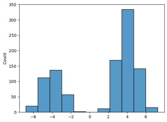
This plot represents the data distribution, i.e., $q(x_0)$. As you can see, our training dataset contains samples from a mixture of two Gaussian distributions, where the component on the right is sampled twice as much frequently.
The forward diffusion process is in Equation 2 of the paper:
\[q(x_{1:T}|x_0):=\prod_{t=1}^T q(x_t|x_{t-1})\]with each step adding Gaussian noise:
\[q(x_t|x_{t-1}):=\mathcal{N}(x_t | \sqrt{1-\beta_t}x_{t-1} ; \beta_t I)\]The mean and variance of this distribution is chosen so that the end distribution of $x_T$ after the diffusion process is a zero-mean, unit-variance Gaussian, from which we can easily sample.
This process is easily implemented with a loop:
# we will keep these parameters fixed throughout
TIME_STEPS = 250
BETA = 0.02
def do_diffusion(data, steps=TIME_STEPS, beta=BETA):
    # perform diffusion following equation 2
    # returns a list of q(x(t)) and x(t)
    # starting from t=0 (i.e., the dataset)

    distributions, samples = [None], [data]
    xt = data
    for t in range(steps):
        q = torch.distributions.Normal(
            np.sqrt(1 - beta) * xt,
            np.sqrt(beta)
        )
        xt = q.sample()

        distributions.append(q)
        samples.append(xt)

    return distributions, samples
_, samples = do_diffusion(dataset)
We can visualize the diffusion process by plotting time on the $x$ axis, and the diffused samples on the $y$ axis:
for t in torch.stack(samples)[:, :, 0].T[:100]:
    plt.plot(t, c='navy', alpha=0.1)
plt.xlabel('Diffusion time')
plt.ylabel('Data')
plt.show()
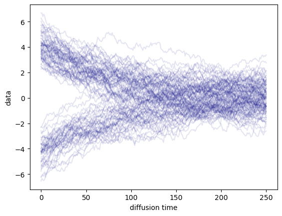
As you can see, adding noise gradually transforms all samples into a Normal $\mathcal{N}(0,1)$ distribution. We are now ready to train a model to invert this process.
Training
To keep things as simple as possible, here we use the loss in Equation 3 in the paper without any of the optimizations presented later, which only play a role for complex, real-world distributions.
In this case, diffusion models are trained by first corrupting the training examples, then trying to reconstruct the cleaner examples from the noisy examples at each step of the corruption process. The loss is an upper bound on the negative log likelihood:
\[L := \mathbb{E}_q\left[ -\log p(x_T) -\sum_{t=1}^T \log\frac{p_\theta(x_{t-1}|x_t)}{q(x_t|x_{t-1})} \right]\]Where the generative model, also called reverse process, has form:
\[p_\theta(x_{t-1}|x_t):=\mathcal{N}(x_{t-1} ; \mu_\theta(x_t,t), \Sigma_\theta(x_t, t))\]Note that we are training two neural networks, $\mu_\theta$ and $\Sigma_\theta$, which take as input a noisy sample $x_t$ and the step $t$, and try to predict the parameters of the distribution of the sample $x_{t-1}$ to which noise was added. Intuitively, we are training these networks to maximize the predicted probability of observing the uncorrputed example $x_{t-1}$ based on $x_t$, i.e., the term $p_\theta(x_{t-1}\vert x_t)$ in the loss, for each diffusion step. Remember that $x_t$ was generated earlier from $x_{t-1}$ by adding noise; the networks have to learn to undo the noise. The other terms in the loss involving $q(x_t\vert x_{t-1})$ are not necessary to learn a good generative model, since they are constant, but are useful as a “frame of reference” to make a “perfect” generative model achieve a loss of 0.
The loss is implemented in the function below. This function requires the entire diffusion trajectory for the training samples, as well as the two neural networks that define the inverse process:
def compute_loss(forward_distributions, forward_samples, mean_model, var_model):
    # here we compute the loss in equation 3
    # forward = q , reverse = p

    # loss for x(T)
    p = torch.distributions.Normal(
        torch.zeros(forward_samples[0].shape),
        torch.ones(forward_samples[0].shape)
    )
    loss = -p.log_prob(forward_samples[-1]).mean()

    for t in range(1, len(forward_samples)):
        xt = forward_samples[t]         # x(t)
        xprev = forward_samples[t - 1]  # x(t-1)
        q = forward_distributions[t]    # q( x(t) | x(t-1) )

        # normalize t between 0 and 1 and add it as a new column
        # to the inputs of the mu and sigma networks
        xin = torch.cat(
            (xt, (t / len(forward_samples)) * torch.ones(xt.shape[0], 1)),
            dim=1
        )
        # compute p( x(t-1) | x(t) ) as equation 1
        mu = mean_model(xin)
        sigma = var_model(xin)
        p = torch.distributions.Normal(mu, sigma)

        # add a term to the loss
        loss -= torch.mean(p.log_prob(xprev))
        loss += torch.mean(q.log_prob(xt))

    return loss / len(forward_samples)
Let us now define two very simple neural networks to predict the mean and variance. Both of these networks take two inputs: the noisy sample $x_t$ and the normalized time-step $t$. As you can see from the snippet above, the time-step is added as an additional column feature, and, since the input is also one-dimensional, the total input size is two.
mean_model = torch.nn.Sequential(
    torch.nn.Linear(2, 4), torch.nn.ReLU(),
    torch.nn.Linear(4, 1)
)
var_model = torch.nn.Sequential(
    torch.nn.Linear(2, 4), torch.nn.ReLU(),
    torch.nn.Linear(4, 1), torch.nn.Softplus()
)
Let’s now train them:
optim = torch.optim.AdamW(
    itertools.chain(mean_model.parameters(), var_model.parameters()),
    lr=1e-2, weight_decay=1e-6,
)
loss_history = []
bar = tqdm(range(1000))
for e in bar:
    forward_distributions, forward_samples = do_diffusion(dataset)

    optim.zero_grad()
    loss = compute_loss(
        forward_distributions, forward_samples, mean_model, var_model
    )
    loss.backward()
    optim.step()

    bar.set_description(f'Loss: {loss.item():.4f}')
    loss_history.append(loss.item())
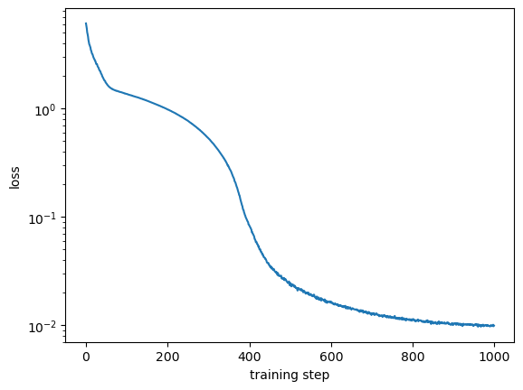
We can make sure that the model has converged by inspecting the loss:
plt.plot(loss_history)
plt.yscale('log')
plt.ylabel('Loss')
plt.xlabel('Training step')
plt.show()
Sample generation
Finally, with the trained neural networks, we can generate new samples from the data distribution.
This process is very similar to the earlier diffusion process, except that here we start from a Normally-distributed $x_T$ and use the predicted mean and variance to gradually “remove” noise:
def sample_reverse(mean_model, var_model, count, steps=TIME_STEPS):
    p = torch.distributions.Normal(torch.zeros(count, 1), torch.ones(count, 1))
    xt = p.sample()
    sample_history = [xt]
    for t in range(steps, 0, -1):
        xin = torch.cat((xt, t * torch.ones(xt.shape) / steps), dim=1)
        p = torch.distributions.Normal(
            mean_model(xin), var_model(xin)
        )
        xt = p.sample()
        sample_history.append(xt)
    return sample_history
samps = torch.stack(sample_reverse(mean_model, var_model, 1000))
for t in samps[:,:,0].T[:200]:
    plt.plot(t, c='C%d' % int(t[-1] > 0), alpha=0.1)
plt.xlabel('Generation time')
plt.ylabel('Data')
plt.show()
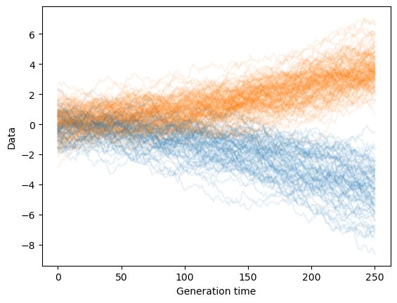
And this is the distribution at the last step of generation:
sns.histplot(samps[-1, :, 0])
plt.show()
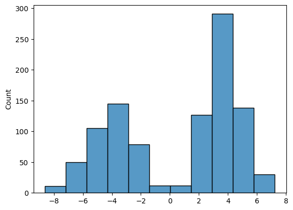
It is very similar to the initial data distribution, which means that our model has successfully learned to generate samples resembling the training dataset!
I hope you found this tutorial useful! You can download a notebook with this code here.