Simplest implementation of LDA topic modeling with collapsed Gibbs sampling
Latent Dirichlet Allocation (LDA) is a classic machine learning algorithm for topic modeling. Topic modeling is an unsupervised approach that discovers hidden topics behind a collection of documents, dividing for example sport news from food recipes and movie reviews. While the math can get complicated, the implementation is surprisingly simple. Let’s dive in!
The model
LDA takes as input a number of documents, each of which is a sequence of words, and tries to assign a “topic” to each word of each document. In this context, a topic is just a probability distribution over words, such that, for example, the topic “soccer” would assign high probability to words like “referee”, “goal” and “ball”, and low probability to words like “cabbage”, “Saturn”, etc. Crucially, LDA does not assign names to the topics it finds, it is up to the user to interpret the resulting topics and assign meaning to them, and in practice this can be rather challenging.
The model behind LDA is typically depicted using a graphical model like this:
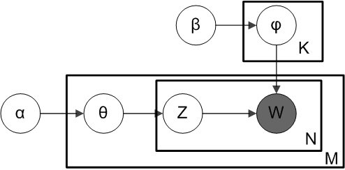
Where $M$ is the number of documents, $N$ the number of words in a document, and $K$ the number of topics, which has to be specified before fitting the model. Each circle is a random variable, and the boxes contain families random variables. In plain terms, this means that the model contains the variables $\phi_1,\ldots,\phi_K$ and $\theta_1,\ldots,\theta_M$ as well as $Z_{m,n}$ and $W_{m,n}$ for $1\leq m\leq M$ and $1\leq n\leq N$, with $Z_{m,n}\in1,\ldots,K$ and $W_{m,n}\in 1,\ldots,R$. Variables are connected by arrows if there is a direct causal relationship between them, that is, if we need the value of one variable to generate the other one (this will become clear in a second).
Each variable $\phi_k$ indicates the probability distribution of words for topic $k$, and follows a Dirichlet distribution: $\phi_k\sim\text{Dirichlet}(\beta)$ The Dirichlet distribution is used for vectors that need to sum to one, in our case probabilities over words, meaning that $\phi_{k,r}$ is the probability of observing the word $r$ in an article about topic $k$. The parameter $\beta$ can be used to bias these probabilities in certain ways, for example to be sharp or diffuse, to be uniform or to favor certain words over others, etc. The variables $\theta_m$ follow a similar distribution: $\theta_m\sim\text{Dirichlet}(\alpha)$ and are used to denote the distribution of topics for each document $m$, so that $\theta_{m,k}$ is the probability of observing a word about topic $k$ in article $m$.
Each word in each document is associated with two variables: $W_{m,n}$ is the word itself that we observe in the dataset (this is the meaning of the gray circle), and $Z_{m,n}$ is the hidden topic that “generated” this word. This means that, given that the topic $Z_{m,n}$ is $z$, the word $W_{m,n}$ is randomly sampled from $\phi_z$, while the topic $Z_{m,n}$ is itself sampled from $\theta_m$. Both topics and words follow categorical distributions parameterized by the respective topic probabilities, that is, $Z_{m,n}\sim\text{Categorical}(\theta_m)$ and $W_{m,n}\sim\text{Categorical}(\phi_{Z_{m,n}})$.
As you can see, this model treats documents as bag-of-words, meaning that there is no sequence relation between words of the same document; We could randomly shuffle all words in a document and the model would not be able to tell that the documents are now gibberish (what do you expect from a model that was introduced in 2003?). The challenge is that, obviously, our dataset only comes with documents and words, all topics are latent (hidden, unknown). This is why we need an inference procedure: to find the values of these latent variables.
But first, let us generate some synthetic data following this model!
import numpy as np
import matplotlib.pyplot as plt
NUM_TOPICS = 3   # K
VOCAB_SIZE = 9   # R
NUM_DOCS = 50    # M
DOC_LENGTH = 50  # N
SEED = 2357

rng = np.random.default_rng(SEED)
We start by creating the topic priors, which indicate the proportion of random documents what will be generated for each topic:
topic_prior = np.arange(1, NUM_TOPICS + 1)**2
topic_prior = topic_prior / topic_prior.sum()
topic_prior
array([0.07142857, 0.28571429, 0.64285714])
In this case, we have three topics with the first being the least likely and the last the most likely.
Next, we define word priors that indicate, for each topic, which words are the more or less likely:
word_weights = [
    np.array([
        6 if i <= j / NUM_TOPICS < i + 1 else 1
        for j in range(VOCAB_SIZE)
    ])
    for i in range(NUM_TOPICS)
]
word_prior = np.vstack([p / p.sum() for p in word_weights])
plt.matshow(word_prior, vmin=0, vmax=1, cmap="bwr")
plt.xlabel('Word')
plt.ylabel('Topic')
plt.colorbar(label="Probability")
plt.title("Word Probability by Topic")
plt.show()
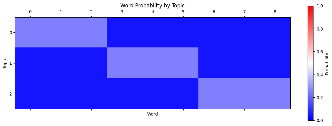
As you can see, each topic is more likely to contain certain “blocks” of words. Note that all words have at least a small probability of appearing in a certain topic.
We can now generate the documents by sampling from these distributions:
documents, document_topics, word_topics = [], [], []
for _ in range(NUM_DOCS):
    # choose the topics in this document
    doc_topic_dist = rng.dirichlet(topic_prior)
    document_topics.append(doc_topic_dist)

    # now sample each word in the document
    doc, doc_word_topics = [], []
    for _ in range(DOC_LENGTH):
        # choose the topic for this specific word
        topic = rng.choice(NUM_TOPICS, p=doc_topic_dist)

        # then choose the word based on this topic
        word = rng.choice(VOCAB_SIZE, p=word_prior[topic])

        doc_word_topics.append(topic)
        doc.append(word)

    word_topics.append(doc_word_topics)
    documents.append(doc)

documents = np.array(documents)
doc_topics = np.array(document_topics)
word_topics = np.array(word_topics)
Here are the first three documents, where each number corresponds to the index of a word in a fictitious dictionary:
documents[:3]
array([[8, 4, 4, 6, 4, 8, 5, 3, 5, 4, 4, 0, 3, 3, 8, 5, 5, 6, 8, 6, 1, 7,
        5, 0, 4, 3, 8, 8, 4, 2, 3, 3, 6, 6, 0, 2, 0, 5, 3, 5, 6, 7, 8, 8,
        6, 8, 5, 8, 1, 0],
       [8, 6, 6, 7, 7, 3, 7, 8, 8, 1, 6, 6, 7, 4, 7, 8, 1, 7, 6, 6, 4, 8,
        7, 8, 8, 8, 8, 4, 7, 8, 8, 7, 6, 7, 2, 2, 0, 7, 8, 6, 7, 3, 8, 7,
        7, 8, 2, 8, 6, 6],
       [7, 6, 6, 5, 5, 5, 6, 8, 6, 4, 7, 5, 6, 7, 4, 3, 4, 5, 5, 6, 5, 7,
        4, 8, 5, 7, 2, 5, 7, 4, 8, 8, 4, 5, 8, 5, 3, 8, 3, 4, 4, 1, 6, 6,
        5, 6, 8, 6, 8, 6]])
And here are the topic probabilities that were used to generate these documents:
doc_topics[:3]
array([[1.96599233e-09, 6.42545804e-01, 3.57454194e-01],
       [4.16229039e-03, 2.71805030e-04, 9.95565905e-01],
       [1.27895936e-12, 5.11000704e-01, 4.88999296e-01]])
For example, the first document is made for 64% of the second topic, which tends to contain words 3, 4 and 5, and for 36% of topic three, which contains words 6, 7 and 8. This is reflected in the word frequency above.
Inference
Inference is the procedure used to find values for latent variables and parameters given the dataset we have. In general there are several ways to do this, be it variational inference, expectation maximization, Monte Carlo methods, etc. In this case, we are going to rely on this latter category and in particular we will be using an algorithm called Gibbs sampling.
Monte Carlo methods give a number of samples from the posterior, in our case $p(Z\vert W)$, which one can then aggregate to find expectations and variances. Markov Chain Monte Carlo (MCMC) methods start from an initial sample, that is, values for latent variables, and updates it in a certain way based to find the next sample, repeating this process thousands of times. This sequential process is what “Markov Chain” means, and as you can imagine lots of variants exist depending on how exactly the samples are updated.
Gibbs sampling is a simple MCMC algorithm that updates one variable at a time based on the value of all other variables. The procedure to take $T$ samples from the posterior is as follows (for simplicity we index $Z$ with $i$ rather than $m$ and $n$):
- Randomly construct a guess $Z^{(0)}$
- For each sampling step $t\in[1,\ldots,T]$:
- For each variable $i\in[1,\ldots,I]$:
- Sample $Z_i^{(t+1)}$ from $p(\cdot \vert Z_1^{(t+1)},\ldots,Z_{i-1}^{(t+1)}, Z_{i+1}^{(t)},\ldots,Z_{I}^{(t)}, W)$
- Store $Z^{(t+1)}$
- For each variable $i\in[1,\ldots,I]$:
- Analyze the samples $Z^{(1)},\ldots,Z^{(T)}$
As you can see, each sample is constructed incrementally by sampling the first variable, then the second variable, etc., until all variables are updated.
To apply this algorithm to LDA, we need to find $p(Z_{m,n}\vert Z_{-(m,n)}, W, \theta, \phi, \alpha, \beta)$, where $Z_{-(m,n)}$ indicates all $Z$ variables except for $Z_{m,n}$, and $\phi$ and $\theta$ are shorthands for $\phi_1,\ldots,\phi_K$ and $\theta_1,\ldots,\theta_M$. This expression can be simplified by integrating away (or “collapsing”) $\theta$ and $\psi$ and instead working with
\[p(Z_{m,n}\vert Z_{-(m,n)}, W, \alpha, \beta) =\int p(Z_{m,n}\vert Z_{-(m,n)}, W, \theta, \phi, \alpha, \beta)p(\theta\vert\alpha)p(\phi\vert\beta)\text{d}\theta\text{d}\phi\]giving rise to what is called collapsed Gibbs sampling. Actually finding this distribution takes a bit of work; The derivation on Wikipedia is rather involved, but not particularly difficult to follow once somebody shows it to you.
Here we are going to skip this and directly look at the result.
Before that, though, let me make our terminology a bit more precise: Each document in the dataset is a sequence of tokens, and each token is one of a number of words.
This means that, for example, the document [2, 1, 2] contains three tokens, and the first and third tokens corresponding to the word with index 2.
Let $W_{m,n}=v\in[1,\ldots,R]$ be the observed token at position $n$ of document $m$, and $Z_{m,n}\in[1,\ldots,K]$ the latent topic that generated this token. The posterior distribution of the corresponding latent topic is
\[p(Z_{m,n}=k\vert Z_{-(m,n)}, W;\alpha,\beta) \propto \left( n^{k,-(m,n)}_{m,(\cdot)}+\alpha_k \right) \frac{ n^{k,-(m,n)}_{(\cdot),v}+\beta_v }{ \sum_{r=1}^V n^{k,-(m,n)}_{(\cdot),r}+\beta_r }\]where $\propto$ means “proportional to”, meaning that the normalization constant is missing, $n_{j,r}^{k,-(m,n)}$ is the number of tokens in the $j$-th document with the $r$-th word symbol assigned to the $k$-th topic, without counting $Z_{m,n}$ itself, $(\cdot)$ indicates summations over the index that it replaces, and $V$ is the number of tokens in a document.
While the notation is rather heavy, all these terms are actually really simple: without counting the $n$-th token in document $m$,
- $n^{k,-(m,n)}_{m,(\cdot)}$ is the number of tokens in document $m$ assigned to topic $k$
- $n^{k,-(m,n)}_{(\cdot),v}$ is the number of tokens with word $v$ assigned to topic $k$
- $\sum_{r=1}^V n^{k,-(m,n)}_{(\cdot),r}$ is the total number of tokens assigned to topic $k$
and where the priors $\alpha$ and $\beta$ just act as additional pseudo-counts.
How can you interpret this formula? The probability that a token in a document belongs to a certain topic is proportional to the number of other tokens in the same document belonging to that topic. That is, the more frequently a topic appears in a document, the more likely that a specific token was also generated from that topic. This probability is then further increased or decreased depending on whether, over the entire dataset, tokens with this word are more frequently assigned to that topic compared to other topics. That is, the more frequently a word is assigned to this topic is across the entire dataset, the more likely that this token was also generated from this topic.
Implementation
Starting from the top, here is a skeleton implementation of Gibbs sampling for LDA:
def sample(ws, zs_initial, n_steps, alpha, beta, rng):
    samples = []

    zs = zs_initial
    for t in range(n_steps):
        zs = np.copy(zs)

        for doc_id in range(ws.shape[0]):
            for word_id in range(ws.shape[1]):
                # find posterior distribution
                p_z_mn = compute_p_z_mn(ws, zs, doc_id, word_id, alpha, beta)

                # sample a new topic according to this distribution
                z_mn = rng.choice(NUM_TOPICS, p=p_z_mn)

                # update the topic assignment
                zs[doc_id, word_id] = z_mn

        # store for later analysis
        samples.append(zs)

    return samples
We simply iterate over all latent variables $Z$ (the specific order does not matter), find out their posterior distribution conditioned on everything else, take a sample from it, update the topic assignments, and repeating this over and over until we are happy. Here, $\alpha$ and $\beta$ are prior topic probabilities that we can use to steer the sampling procedure if we have external domain knowledge about the domain from where we collected the dataset, and if the dataset itself does not contain enough information to contradict this knowledge. In our case, although we know how the topic distribution, we do not want to introduce any additional information, therefore we will use diffused and non-informative priors.
The posterior computation, while mathematically involved to derive, is also very simple to implement:
def compute_p_z_mn(ws, zs, doc_id, word_id, alpha, beta):
    """
    Compute the probability of each topic for a given word in a document.

    Parameters
    ----------
    ws : np.ndarray
        Array of shape (NUM_DOCS, DOC_LENGTH) containing the observed word
        indices for each document.
    zs : np.ndarray
        Array of shape (NUM_DOCS, DOC_LENGTH) containing the current topic
        assignments for each word in each document.
    doc_id : int
        Index of the document being updated (m in the formula above).
    word_id : int
        Index of the word within the document being updated (n in the formula
        above).
    alpha : np.ndarray
        Dirichlet prior for topic distribution per document, shape
        (NUM_TOPICS,).
    beta : np.ndarray
        Dirichlet prior for word distribution per topic, shape (VOCAB_SIZE,).

    Returns
    -------
    np.ndarray
        Array of shape (NUM_TOPICS,) containing the probability of each topic
        for the given word position.
    """

    # overwrite the topic of the word in consideration to make sure that it is
    # not used in the calculations
    z_mn = zs[doc_id, word_id]
    zs[doc_id, word_id] = -1

    # this is the observed word
    v = ws[doc_id, word_id]

    # compute the unnormalized probability of each topic
    topic_probabilities = np.zeros(NUM_TOPICS)
    for k in range(NUM_TOPICS):
        # find which words are assigned to topic k
        has_topic_k = zs == k

        # number of word in document doc_id assigned to topic k
        front = alpha[k] + np.sum(has_topic_k[doc_id])

        # number of times token v was assigned to topic k
        numerator = beta[v] + np.sum((ws == v) & has_topic_k)

        # total number of words assigned to topic k
        denominator = np.sum(beta) + np.sum(has_topic_k)

        # unnormalized probability of topic k for word_id in doc_id
        topic_probabilities[k] = front * numerator / denominator

    # restore the previous latent topic assignment
    zs[doc_id, word_id] = z_mn

    # normalize probabilities so they sum to one
    return topic_probabilities / topic_probabilities.sum()
There is one last step before we can run this algorithm: we need to compute the log likelihood of the current solution. This is useful, together with several other checks, to make sure that the algorithm converged and that the samples are independent and identically distributed (i.i.d.), meaning that they can be analyzed to produce reliable conclusions.
The log-likelihood of the LDA model is:
\[\log p(W, Z, \theta, \phi ; \alpha, \beta) = \sum_{k=1}^K \log p(\phi_k ; \beta) + \sum_{m=1}^M \left[ \log p(\theta_m ; \alpha) + \sum_{n=1}^N \left[ \log p(Z_{m,n} \vert \theta_m) + \log p(W_{m,n} \vert \phi, Z_{m,n}) \right] \right]\]Where:
- $p(\phi_k ; \beta)\sim\text{Dirichlet}(\beta)$ is the word distribution for topic $k$: $p(\phi_k;\beta)\propto\prod_{v=1}^R\phi_{k,v}^{\beta_v-1}$
- $p(\theta_m ; \alpha)\sim\text{Dirichlet}(\alpha)$ is the topic distribution for document $m$: $p(\theta_m;\alpha)\propto\prod_{k=1}^K \theta_{m,k}^{\alpha_k-1}$
- $p(Z_{m,n} \vert \theta_m)\sim\text{Categorical}(\theta_k)$ is the topic of word $n$ in document $m$: $p(Z_{m,n}=k\vert\theta_m)=\theta_{m,k}$
- $p(W_{m,n} \vert \phi, Z_{m,n})\sim\text{Categorical}(\phi_{Z_{m,n}})$ is the word at position $n$ in document $m$: $p(W_{m,n}=v\vert\phi,Z_{m,n}=k)=\phi_{k,v}$
There seems to be a problem, though: we collapsed the topic distributions, meaning that we do not have $\phi$ nor $\theta$ available. Luckily, they can be easily estimated from the topic assignments $Z$. The probability of topic $k$ in document $m$ is
\[\theta_{m,k} \propto \sum_{n=1}^N \mathbb{I}[Z_{m,n}=k ]\]where $\mathbb{I}$ is the indicator function, that is, $\mathbb{I}[P]=1$ if the predicate $P$ is true, otherwise it equals 0. The probability of word $r$ in topic $k$ is
\[\phi_{k,v}\propto \sum_{m=1}^M \sum_{n=1}^N \mathbb{I}[Z_{m,n}=k \land W_{m,n}=v]\]Let’s write a function to compute these two probabilities:
def compute_topic_probabilities(ws, zs):
    # this is theta
    doc_topic_prior = np.array([
        [np.mean((zs[j] == k)) for k in range(NUM_TOPICS)]
        for j in range(NUM_DOCS)
    ])
    # normalize by document (sum over topics is 1)
    doc_topic_prior = (
        doc_topic_prior / doc_topic_prior.sum(axis=1, keepdims=True)
    )

    # this is phi
    word_topic_prior = np.array([
        [np.mean((ws == v) & (zs == k)) for v in range(VOCAB_SIZE)]
        for k in range(NUM_TOPICS)
    ])
    # normalize by topic (sum over words is 1)
    word_topic_prior = (
        word_topic_prior / word_topic_prior.sum(axis=1, keepdims=True)
    )

    return doc_topic_prior, word_topic_prior
Now, we can finally write out the complete function for a single sampling step:
def next_step(ws, zs, alpha, beta, rng):
    doc_topic_prior, word_topic_prior = compute_topic_probabilities(ws, zs)

    # Dirichlet likelihoods without normalization constants (which only depend
    # on alpha and beta)
    loglik = (
        np.sum((alpha - 1) * np.log(1e-6 + doc_topic_prior))
        + np.sum((beta - 1) * np.log(1e-6 + word_topic_prior))
    )

    new_zs = np.copy(zs)
    for doc_id in range(ws.shape[0]):
        for word_id in range(ws.shape[1]):
            # find posterior distribution
            p_z_mn = compute_p_z_mn(ws, new_zs, doc_id, word_id, alpha, beta)

            # sample a new topic according to this distribution
            z_mn = rng.choice(NUM_TOPICS, p=p_z_mn)

            # update the topic assignment
            new_zs[doc_id, word_id] = z_mn

            # likelihood contribution of this word
            pz = doc_topic_prior[doc_id, z_mn]
            pwz = word_topic_prior[z_mn, ws[doc_id, word_id]]
            loglik += pz + pwz

    return new_zs, loglik / (ws.shape[0] * ws.shape[1])
To check the reliability of MCMC samples, it is common to start a few independent runs (also called chains) and compare the resulting likelihoods and parameters: Ideally, there should be no difference between the runs. Because this process is quite time-consuming, we are going to use multi-processing to start several sampling processes in parallel, using a queue to report the sampling status to the master process:
SENTINEL = "DONE"


def sample_one_chain(n_samples, process_id=0, update_queue=None):
    # initial topic priors
    alpha = 0.2 * np.ones(NUM_TOPICS)
    beta = 0.2 * np.ones(VOCAB_SIZE)

    # randomly initialize topic assignments
    rng = np.random.default_rng(SEED + 325 + process_id)
    zs = rng.choice(
        NUM_TOPICS, size=(documents.shape[0], documents.shape[1]),
        p=alpha / alpha.sum()
    )

    logliks, all_samples = [], []
    for t in range(n_samples):
        # update topic assignments
        zs, ll = next_step(documents, zs, alpha, beta, rng)

        # save progress
        all_samples.append(zs)
        logliks.append(ll)

        if update_queue is not None:
            # for multiple processes, we report the progress in the queue
            if t % 10 == 0:
                update_queue.put((process_id, t, ll), block=False)
        elif (t + 1) % 100 == 0:
            # For single-process runs, we just print the current status
            print(f'Step {t + 1:04d} - NLL: {ll:.4f}')

    if update_queue is not None:
        # notify master process that we are done
        update_queue.put(SENTINEL)

    # return samples and likelihoods
    all_samples = np.stack(all_samples)
    return logliks, all_samples
Let’s now write the sampler:
import os
from multiprocessing import Manager
from concurrent.futures import ProcessPoolExecutor, as_completed
from tqdm.notebook import trange


def sample(num_chains, num_samples, num_workers=None):
    if num_workers is None:
        num_workers = min(num_chains, (os.cpu_count() or 2) - 1)

    with Manager() as man:
        with ProcessPoolExecutor(max_workers=num_workers) as executor:
            # start the processes
            update_queue = man.Queue()
            futures, progress_bars = [], []
            for i in range(num_chains):
                futures.append(
                    executor.submit(
                        sample_one_chain, num_samples, i, update_queue
                    )
                )
                progress_bars.append(
                    trange(num_samples, position=i, desc=f'Chain {i + 1}')
                )

            # update the progress bars as long as processes are running
            alive = len(futures)
            while True:
                msg = update_queue.get()
                if msg == SENTINEL:  # a process finished
                    alive -= 1
                    if alive == 0: # all processes finished
                        break
                else:
                    # update bar
                    pid, t, nll = msg
                    progress_bars[pid].update(10)
                    progress_bars[pid].set_postfix({'NLL': nll})

            # collect results
            chain_lls, chain_samples = [], []
            for fut in as_completed(futures):
                nll, all_samples = fut.result()
                chain_lls.append(nll)
                chain_samples.append(all_samples)

    return np.array(chain_lls), np.stack(chain_samples)
Aaand let’s go:
chain_lls, chain_samples = sample(num_chains=4, num_samples=2000)
Chain 1:   0%|██████████| 2000/2000 [09:57<00:00, 3.41it/s, NLL=1.23]


Chain 2:   0%|██████████| 2000/2000 [09:57<00:00, 3.44it/s, NLL=1.17]


Chain 3:   0%|██████████| 2000/2000 [09:57<00:00, 3.37it/s, NLL=1.16]


Chain 4:   0%|██████████| 2000/2000 [09:57<00:00, 3.33it/s, NLL=1.19]
This took about ten minutes. There are definitely many opportunities to make it faster, but here we prioritized clarity.
Let’s first check the log likelihoods:
for i, c in enumerate(chain_lls):
    plt.plot(c, label=f'Chain {i}')

plt.xlabel("Step")
plt.ylabel("Log likelihood")
plt.legend()
plt.show()
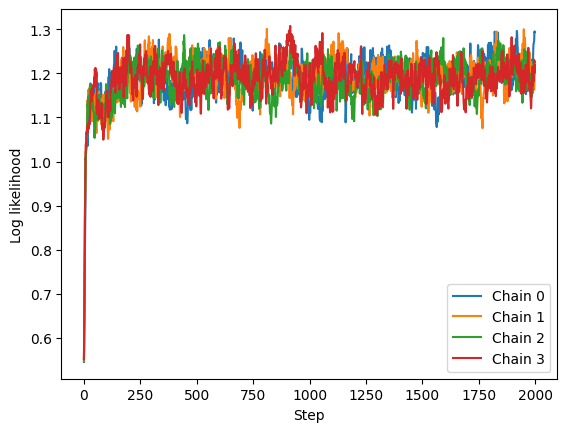
The four chains are indistinguishable, however you do see a few low frequency oscillations, meaning that samples close in time tend to have similar likelihoods. We will leave proper convergence checks for another time, but this is some superficial evidence that the chains converged and the samples are i.i.d. from the posterior.
To further reduce the risk of correlated samples, it is common to discard the first thousands or so (the “burn-in” samples), then only take every $n$-th sample (“thinning” the chain).
samples = chain_samples[:, 500:]  # burn-in
samples = samples[:, ::5]  # thinning
samples.shape  # (num_chains, num_samples, num_docs, doc_length)
(4, 300, 50, 50)
Let us now compute the global topic probabilities. We must do this separately for each chain because the topics are non-identifiable, meaning that there is no way for different chains to agree on what should be the “first topic”, each chain decides this randomly. There are of course ways to enforce identifiability, but they are again out of scope for this post.
np.stack([
    np.mean(samples == k, axis=(1, 2, 3))
    for k in range(NUM_TOPICS)
]).T  # (num_chains, num_topics)
array([[0.58890933, 0.090024  , 0.32106667],
       [0.31869067, 0.59813733, 0.083172  ],
       [0.309356  , 0.601944  , 0.0887    ],
       [0.598616  , 0.090616  , 0.310768  ]])
As you can see, the topic proportions are roughly the same in every chain, but the order of the topics is different.
For reference, the proportion of the actual topics used to generate the dataset are
# observed topic distribution
[
    np.mean(word_topics == k)
    for k in range(NUM_TOPICS)
]
[0.0608, 0.3124, 0.6268]
The inferred probabilities do not exactly match the topic distributions used to generate the dataset (which are unknown in real-world applications), but are a bit more uniform. This is a consequence of our values for the priors $\alpha$ and $\beta$, which tend to favor uniform distributions and thus avoid too skewed probabilities when there is not a lot of data. This is why the first topic has an observed probability of 6% but is inferred at about 9%, and the third topic has a probability of 63% but is inferred at slightly below 60%, while the probability second topic is more or less estimated correctly at 31%. Focusing on the first chain and matching topics by probabilities, the first topic in the chain corresponds to the third topic used to generate the dataset, the second to the first, and the third to the second.
Let’s now look at the first five documents in the dataset. They were generated with this mixture of topics:
def plot_matrix(data, title, xlabel, ylabel):
    fig, ax = plt.subplots(figsize=(6, 3))
    cm  = ax.matshow(data, vmin=0, vmax=1, cmap='bwr')
    fig.colorbar(cm, label='Probability')
    ax.set_xlabel(xlabel)
    ax.set_ylabel(ylabel)
    ax.set_title(title)
    fig.tight_layout()
    fig.show()


plot_matrix(
    np.array([
        [np.mean(word_topics[i] == k) for k in range(NUM_TOPICS)]
        for i in range(5)
    ]).T,
    "Observed Topic Distribution", "Document", "Topic"
)
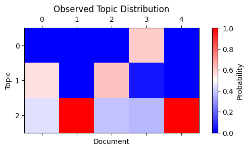
While the first chain assigned the following topics to these documents:
plot_matrix(
    np.stack([
        [np.mean(samples[0, :, i] == k) for k in range(NUM_TOPICS)]
        for i in range(5)
    ]).T,
    "Inferred Topic Distribution (Chain 1)", "Document", "Topic"
)
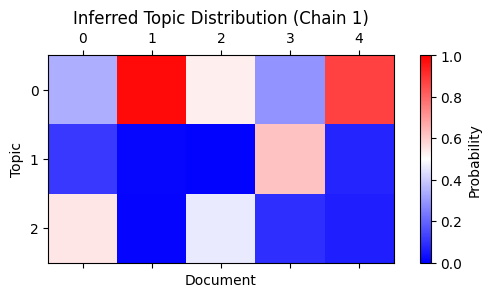
This assignment is correct if you consider the mapping from topics in the first chain to those in the dataset (row 1 goes to 3 , 2 to 1, and 3 to 2), and that these probabilities are smoothed by the priors.
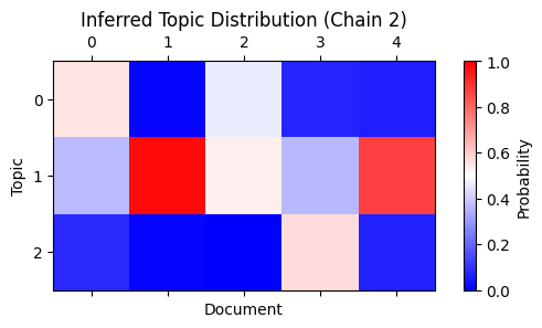
The second chain has a different topic assignment, but the probabilities again match after permuting the rows appropriately (1 to 2, 2 to 3, and 3 to 1):
plot_matrix(
    np.stack([
        [np.mean(samples[1, :, i] == k) for k in range(NUM_TOPICS)]
        for i in range(5)
    ]).T,
    "Inferred Topic Distribution (Chain 2)", "Document", "Topic"
)
Conclusion and next steps
We just implemented the collapsed Gibbs sampling algorithm for the LDA topic model and applied it successfully to a toy dataset. While we only scratched the surface of a number of deep and complex topics, I hope that this implementation and explanation was simple enough for you to follow and understand.
So what is topic modeling useful for in an era dominated by large language models and reasoning agents? It turns out that, while the inspiration for this algorithm comes from natural language, documents and words, the same concepts can be used for any domain which contains “objects” that are composed of simpler “units”, and different types of objects have different unit composition. For example, this paper treats patients as documents and diseases as words, and uses topic modeling to find multimorbidities, groups of diseases that frequently occur together. Further analysis revealed novel associations between genetic information of the patients and the topics they were assigned to, and found that the topic assignment made it easier to predict the risk of developing certain conditions. That paper is also interesting in that it does not treats diseases as completely independent, but rather it uses a pre-defined disease ontology to make the model more likely to assign similar diseases to similar topics.
Quite an interesting application, if you ask me. Now go ahead and try to find other interesting applications for topic modeling!